Machine Learning
Having studied search algorithms, learning to deal with real-world uncertainties, and learning from experience - in the final section of this course, we turn our attention to learning from data. A series of algorithms classified as machine learning models, our goal is to enable computers to learn from and make predictions or decisions based on data. Machine learning models are often classified into supervised learning and unsupervised learning. In supervised learning, models are trained on labeled data, where the input and output are known. In unsupervised learning on the other hand, models are trained on unlabeled data, and the goal is to discover patterns or relationships in the data. Reinforcement learning may also be thought of as a form of machine learning, where the data is generated through interactions with an environment.
Gradient Descent
If most of AI could be summarized as a single mathematical process, it would be gradient descent. Be it reinforcement learning, machine learning, or constraint satisfaction, our solution approach usually takes the form of starting with an initial guess, and iteratively, but cleverly, making changes to it until some desired properties emerge. Recall our discussion of hill climbing approaches, and think about how you would extend this idea to continuous domains? For instance, how would you use hill climbing to find the minimum point of the function, $y = x^2$?
A useful measure that can help us to take hill-climbing steps in the right direction as well as inform how big of a step we should take is the rate of change of an objective function with respect to its inputs. For a univariate function, this quantity is known as the derivative of the function with respect to its inputs. For multivariate function, this is known as the gradient of the objective function, which is simply a collection of derivatives with respect to every variable that the objective is a function of. The gradient is a vector that points in the direction of the greatest rate of increase of the objective function. The gradient is also perpendicular to the contour lines of the objective function. Depending on whether our problem is one of maximization or minimization, we take steps either towards the gradient's direction (direction of steepest ascent), or away from it (direction of steepest descent).
In general, given a function $f$ of $n$ variables, the gradient of $f$ is defined as follows: $$\nabla f = \left[\frac{\partial f}{\partial x_1}, \frac{\partial f}{\partial x_2}, \cdots, \frac{\partial f}{\partial x_n}\right]$$ where $\frac{\partial f}{\partial x_i}$ is the partial derivative of $f$ with respect to the function input $x_i$. For example, let $f(x,y) = x^2 + y^2$. The partial derivative of the objective function with respect to $x$ (i.e., $\frac{\partial f}{\partial x}$) can be solved using the chain rule as follows: $$\frac{\partial f}{\partial x} = \frac{\partial f}{\partial x}\frac{\partial x}{\partial x} + \frac{\partial f}{\partial y}\frac{\partial y}{\partial x} = 2x(1) + 2y(0) = 2x$$ Similarly, $\frac{\partial f}{\partial y} = 2y$. Therefore, $\nabla f = \left[2x, 2y\right]$.
In order to maximize a function $f$ of $n$ variables, we can take a step in the direction of the gradient of $f$ at the current point. This is known as gradient ascent. Similarly, in order to minimize a function $f$ of $n$ variables, we can take a step in the direction opposite to the gradient of $f$ at the current point. This is known as gradient descent. Let $\mathbf{x}$ be a vector of $n$ variables, let $f$ be a function of $\mathbf{x}$, and let $\alpha$ be the learning rate. The gradient descent algorithm can be summarized as follows:
function GRADIENT-DESCENT(f, 𝐱, alpha, threshold):
    while True:
        gradient = calculate_gradient(f, 𝐱)
        if magnitude(gradient) < threshold:
                return 𝐱
𝐱 = 𝐱 - α * gradient𝐱 = 𝐱 + α * gradientFor a refresher on how to compute derivates, partial derivates and gradients, please refer to Chapter 5 of Mathematics for Machine Learning.
Here, instead, we focus our attention to one specific method of computing gradients of composite functions using the chain rule. The chain rule is a fundamental concept in calculus that allows us to compute the derivative of a composite function. For example, let $f(x) = g(h(x))$. The chain rule states that the derivative of $f$ with respect to $x$ is given by: $$\frac{df}{dx} = \frac{dg}{dh}\frac{dh}{dx}$$ This can be extended to multivariate functions. Let $f(x,y) = g(h(x,y))$. The chain rule states that the partial derivative of $f$ with respect to $x$ is given by: $$\frac{\partial f}{\partial x} = \frac{\partial g}{\partial h}\frac{\partial h}{\partial x}$$ And the partial derivative of $f$ with respect to $y$ is given by: $$\frac{\partial f}{\partial y} = \frac{\partial g}{\partial h}\frac{\partial h}{\partial y}$$ Indeed, this is exactly what we did in the earlier example to compute the gradient of $f(x,y) = x^2 + y^2$. We computed the partial derivative of $f$ with respect to $x$ and $y$, and combined them to get the gradient of $f$. In class, we discussed how many problems in AI boil down to defining our goals as objective functions that we want to maximize or minimize. In many such cases, we can use gradient descent to find the optimal solution. For example, in the case of linear regression, we can use gradient descent to find the optimal values of the parameters that minimize the Mean Squared Error across all data points. Now, you may notice that the gradient descent algorithm is an iterative one, i.e., we need to recompute the derivatives/gradients after every update to our set of parameters. This can be computationally expensive, especially when the number of variables is large. However, modern machine learning toolkits such as PyTorch do this with seemingly little effort! How does this work then?
In order to efficiently compute derivatives of complicated objective functions, we rely on an internal representation of the objective function in the form of a computational graph. A computational graph is a directed graph that represents the flow of data through a series of operations. Each node in the graph represents an operation (as well as the partial function value evaluated upto that operation), and each edge represents the flow of data from one operation to another. The graph is constructed by breaking down the objective function into a series of elementary operations, and connecting them in the order in which they are executed. The graph, when traversed in a depth-first manner, allows us to compute the objective function value by applying the operations in the correct order.
Building such a graph allows us to compute the derivative of the objective function with respect to its inputs by applying the chain rule in a reverse order through the graph. This process is known as automatic differentiation, and is central to modern machine learning frameworks. Let's take an example, and explore how we can construct a computation graph by splitting the function by operators. Consider the function $f(x,y) = (x+y)^2$. We can split this function into elementary operations as $f(x,y) = (x+y) \times (x+y)$. We then look at the 'outermost' operator - in other words, the operator that is applied at the final stage of the function evaluation. In this case, it's the multiplication operator, that takes two inputs and multiplies them. In our case, both inputs are the same, i.e., $(x+y)$. Now, we split each $(x+y)$ by the addition operator, which also accepts two inputs, namely $x$ and $y$. We can now construct a computation graph that looks like this:
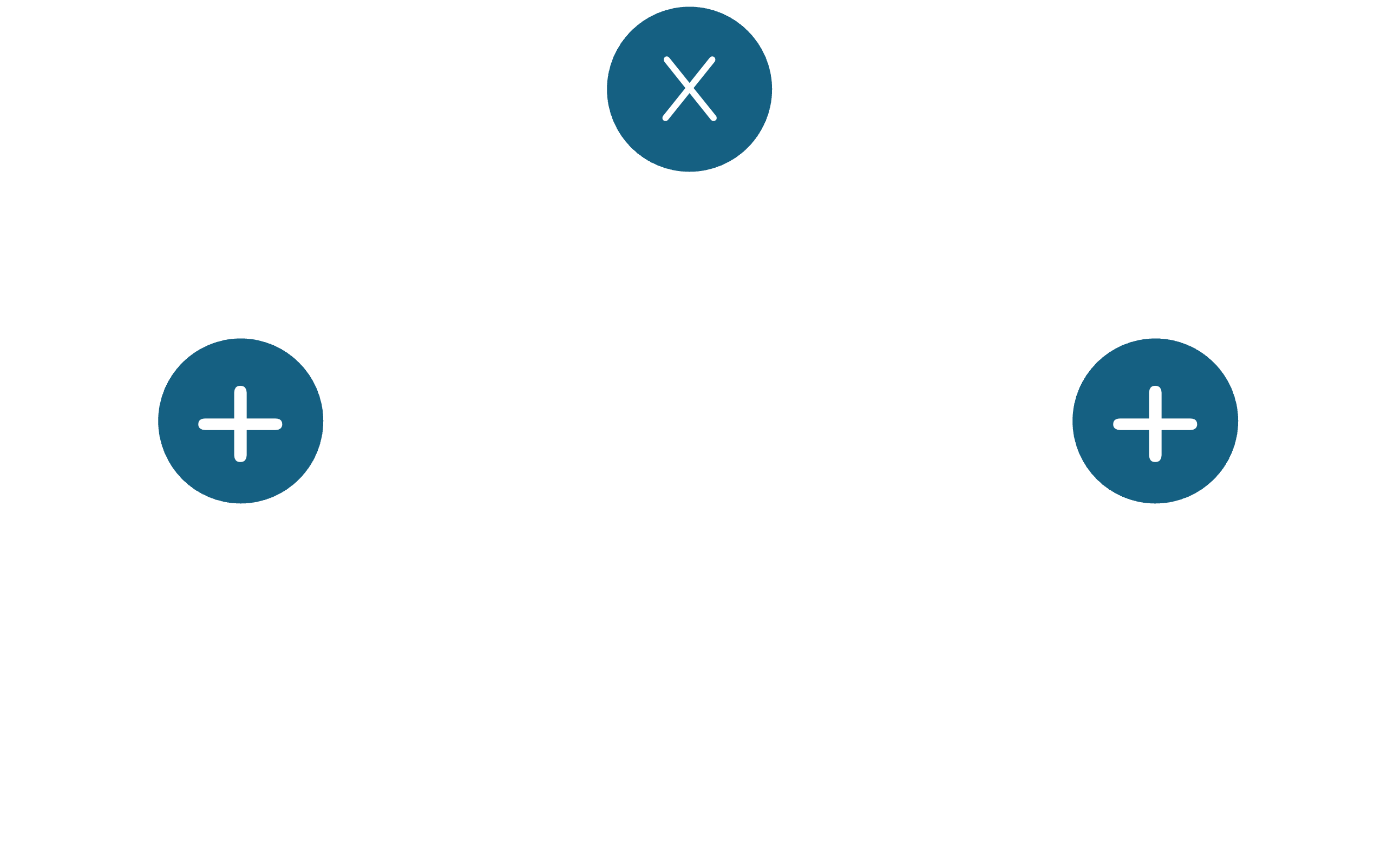
In this graph, each operator node also represents the function below it. For instance, each of the nodes with the $+$ symbol represents the (sub)function $x+y$, and the node with the $\times$ symbol combines these under multiplication to give us our original function $(x+y) \times (x+y)$. The graph is traversed in a forward manner (bottom to top) to compute the function value.
Next, we will extend this graph to compute the derivative of the function with respect to $x$. We can do this by applying the chain rule in a reverse manner through the graph. The chain rule states that the derivative of a composite function is the product of the derivative of the outer function with respect to the inner function, and the derivative of the inner function with respect to the input. Take for instance, our function, $f(x,y) = (x+y)^2$. The derivative of $f$ with respect to $x$ is given by: $$\frac{\partial f}{\partial x} = \frac{\partial f}{\partial (x+y)}\frac{\partial (x+y)}{\partial x}$$ To represent the computation of this derivative on the graph, we label each edge with the partial derivative of the parent node with respect to the input along that edge. For example, $$\frac{\partial f(x,y)}{\partial (x+y)} = (x+y)$$ Similarly, $$\frac{\partial (x+y)}{\partial x} = 1,\quad \textrm{and}\quad \frac{\partial (x+y)}{\partial y} = 1$$ This gives us the following graph:
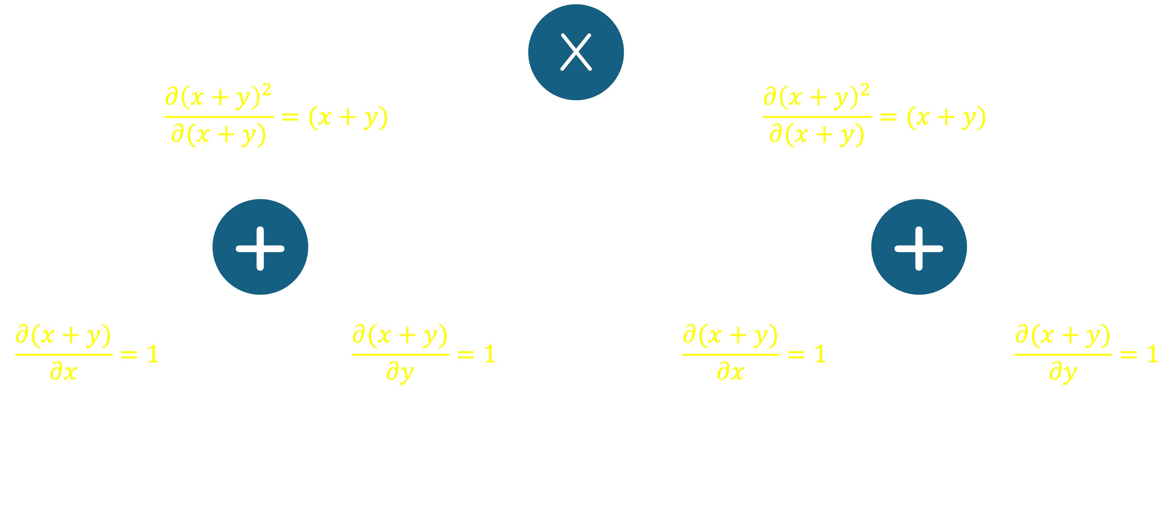
The key benefit of drawing such a graph is that it allows us to compute the derivative of the objective function with respect to any of its inputs by traversing the graph in a top-down fashion, also referred to as backpropagation. To find, for instance, the derivative of $f(x,y)$ with respect to $x$, we first isolate all the paths that go from the root node down to a leaf with a value of $x$. For each path, we multiply the derivatives along the branches that make up the path, and finally sum these values together. In our graph, we have two paths that lead to $x$, starting from the top: reachable by traversing left$\rightarrow$left, or right$\rightarrow$left from the root. For the first path, the derivatives along the branches are $(x+y)$ and $1$ respectively, so multiplying them together gives us $(x+y)$. For the second path, the derivatives along the branches are also $(x+y)$ and $1$ respectively, so multiplying them together once again gives us $(x+y)$. Summing these two values gives us $2(x+y)$, which is the derivative of $f(x,y)$ with respect to $x$.
With a function as simple as our example, the improvements in computational efficiency may not be immediately obvious, but for a more complex function with many variables, the computational savings can be significant. This is because we can reuse the intermediate results of the forward pass to compute the gradients in the backward pass. Further, the graph only needs to be constructed once, and for any value of the function's inputs, we can quickly compute the function value and its gradient. Before we try a more complex example, let's first put together a set of basic rules that we can use to construct these graphs, based on some of the most common elementary operations.
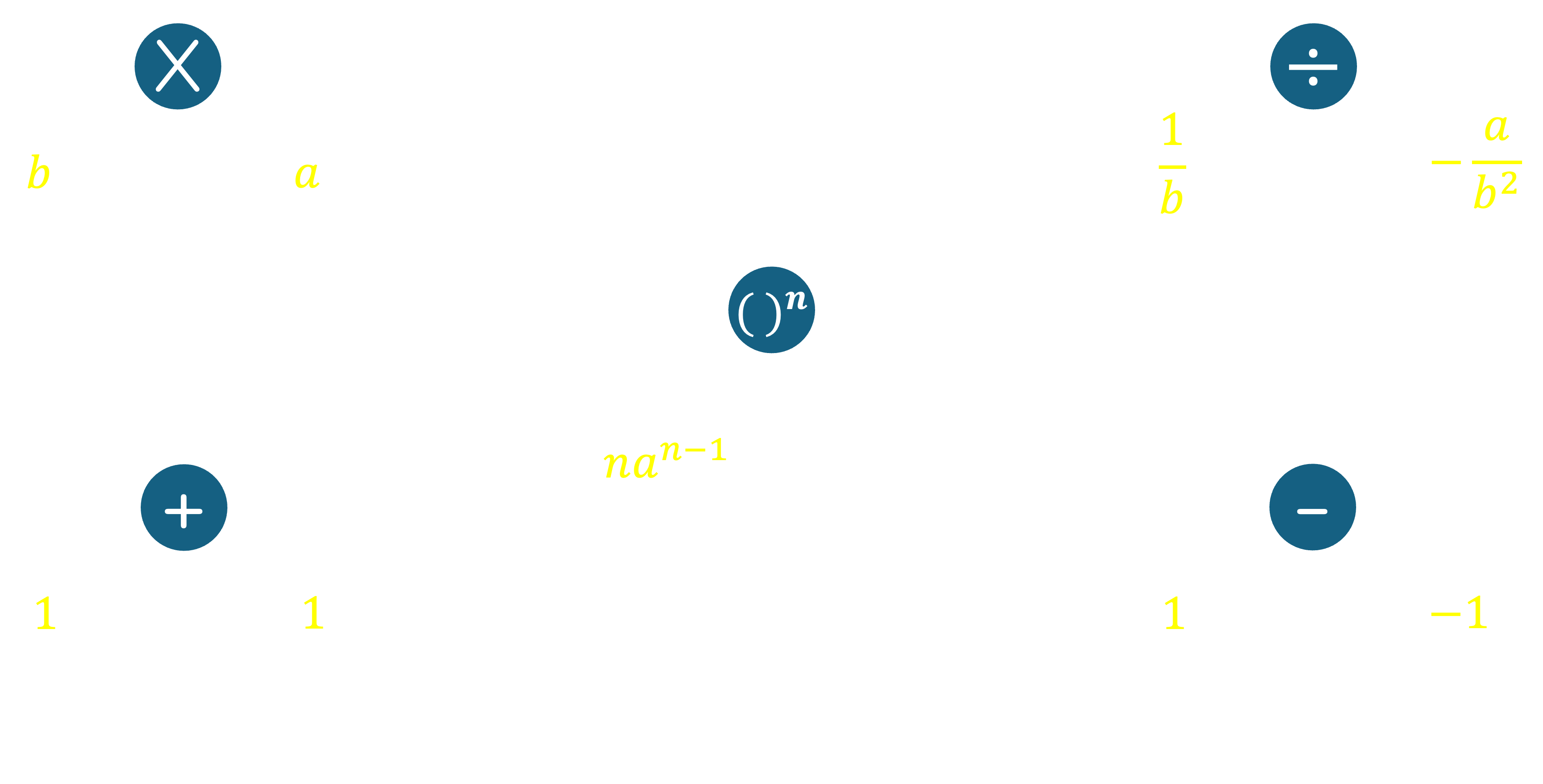
For a multiplication operator, the derivative along one branch is simply the input along the other branch. This is because if $f = ab$, then $\nabla_a f = b$ and $\nabla_b f = a$. For an addition operator, the derivative along both branches is 1. This is because if $f = a+b$, then $\nabla_a f = 1$ and $\nabla_b f = 1$. For subtraction, the derivative along the left branch is 1, and the derivative along the right branch is -1. This is because if $f = a-b$, then $\nabla_a f = 1$ and $\nabla_b f = -1$. For a power operator, the derivative along the base branch is the exponent times the base raised to the power of the exponent minus one. This is because if $f = a^b$, then $\nabla_a f = b \cdot a^{b-1}$. Note that the power operator only takes one input. For a division operator, the derivative along the numerator branch is the reciprocal of the denominator, and the derivative along the denominator branch is the negative of the numerator divided by the square of the denominator. This is because if $f = \frac{a}{b}$, then $\nabla_a f = \frac{1}{b}$ and $\nabla_b f = -\frac{a}{b^2}$.
Let's now take a more complex example to illustrate how we can construct a computation graph and compute the gradient of the objective function with respect to its inputs. Recall the example of Linear Regression in a 2-dimensional space from class, where the objective was to minimize the Mean Squared Error. Let $S$ be the set of points to which we are trying to fit a line, and let the line be given by the equation $y = mx+c$. The objective function was defined as $MSE(m,c) = \frac{1}{|S|}\sum_{(i,j) \in S}(j - (mi+c))^2$. We can construct a computation graph for this function as follows.
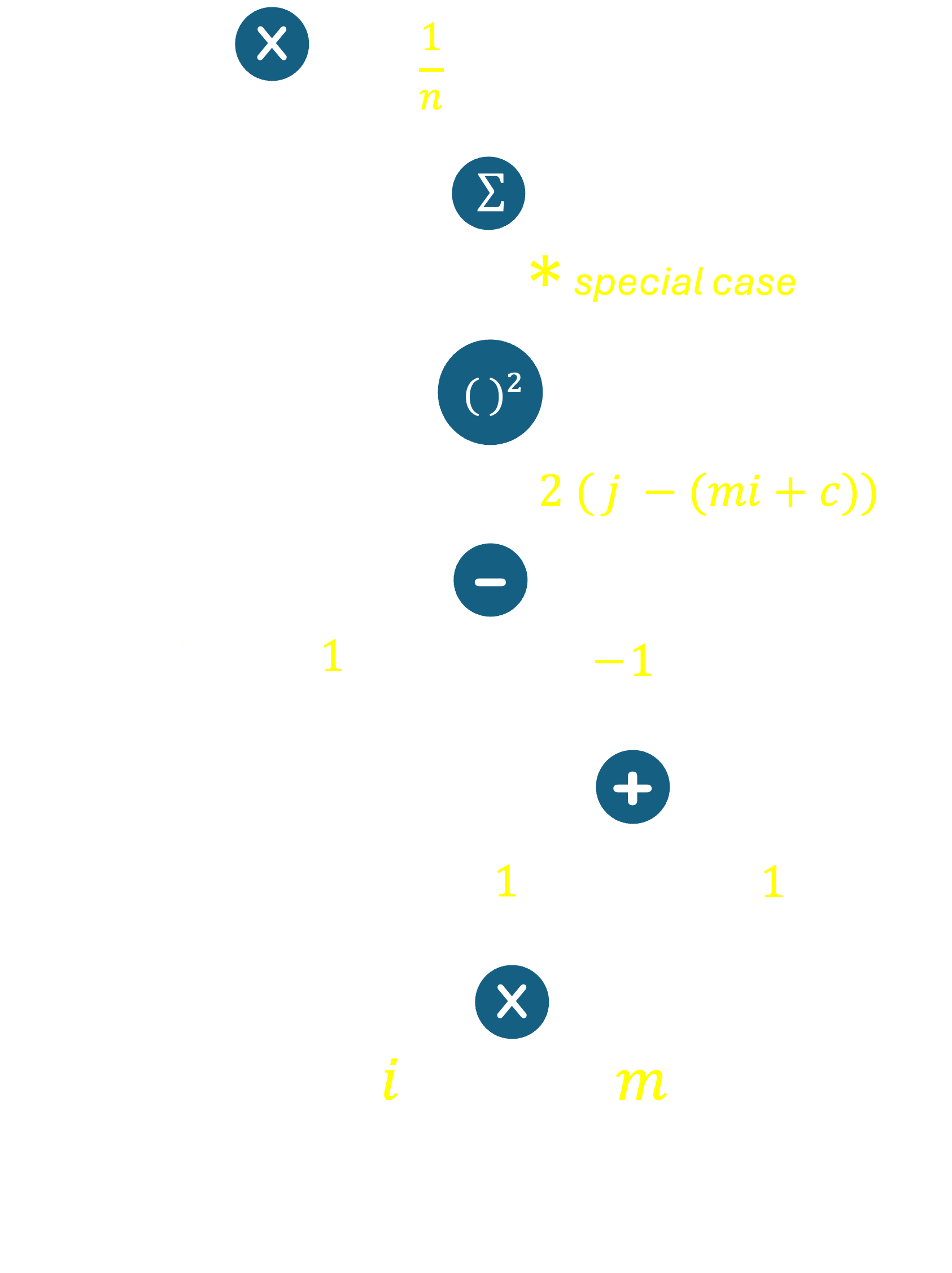
Given what we know about elementary operations from earlier in these notes, most of this graph should be fairly easy to understand. One exception is the summation operator. Recall that a summation operator simply represents a sum of many terms. In our case, the sum operator represents the sum of all the squared errors across all points in our dataset. Here, we recall the sum rule in calculus, which states that the derivative of a sum of functions is the sum of the derivatives of the functions. In other words, $$\frac{\partial}{\partial x}\sum_i f_i(x) = \sum_i\frac{\partial}{\partial x} f_i(x)$$
Armed with this, we can now compute the gradient of the objective function, MSE, with respect to its inputs ($m$ and $c$). From the top of the graph, there is one path that leads us to the leaf node $m$ (in reality there are $|S|$ paths, one for each data point in our data set). Multiplying the derivatives along this branch, and using the sum rule from above, we get: $$\nabla_m MSE(m,c) = \frac{1}{n}\sum_{(i,j)\in S} 2(j-(mi+c))\times -1 \times 1 \times i$$ Similarly, for $c$, we get: $$\nabla_c MSE(m,c) = \frac{1}{n}\sum_{(i,j)\in S} 2(j-(mi+c))\times -1 \times 1$$
Finally, we are ready to solve Linear Regression using Gradient Descent. In order to do so, we start with some initial estimate of $m$ and $c$, say $m=0$ and $c=0$. We then iteratively update $m$ and $c$ using the gradients we computed above. Recall that the update equations are given by: $$m = m - \alpha \nabla_m MSE(m,c)$$ $$c = c - \alpha \nabla_c MSE(m,c)$$ where $\alpha$ is the learning rate. We repeat this process, alternating between updating the slope term $m$ and the intercept term $c$ until the gradients are close to zero, or until we reach a specified number of iterations without much change in our objective function. While we end our discussion of gradient descent here, we will once again, encounter it when we discuss Neural Networks later in the course.
Here's another really nice resource about computation graphs and automatic differentiation: Blog post by Christopher Olah. Please note that there are minor differences between the representations of the computation graph used by Christopher and me. For grading purposes, please use the notation we've discussed in class - reflected in my notes above - in all problem sets.
Feature Extraction, Vector Representations
In machine learning, the first step is to transform raw data at hand into a structured set of informative features that can be fed into algorithms. This process involves selecting key characteristics from the data that are most relevant for the task at hand, often based on domain knowledge, and converting them into numerical representations, which we can then use in order to compute complex relationships. This process is called feature extraction.
There are a host of techniques used for converting raw data into numerical information - and the choice of which to use almost always depends on the problem, the model, and the data distribution. This is best explained with the following example.
Spam Classification: Given a set of emails labeled as spam or ham (not spam), our goal is to build a machine learning algorithm that learns what differentiates spam emails from ham emails, based on a set of features provided to the model. In other words, given some numeric feature information about an email, we want to predict whether it is spam or ham. In order to do so, we must first select the features that are most relevant to the task at hand. If we consider building such a classifier for use at Northeastern University, the following features of an email will likely be useful for the task:
- Domain of the sender's address
- Call to action/sense of urgency
- Presence of attachments
- Presence of links
- Typos in the email
Now given an email, we must convert these features into numerical representations, since the driving idea behind machine learning models is to learn mathematical relationships between the input and output data. Let us now reason about how each of these features can be converted into numerical representations.
Sender Domain: The sender's email address can, in theory, be registered with one of infinitely many email domains. However, not every unique domain is necessarily relevant to the task of spam classification. For instance, the use of a domain such as northeastern.edu or khoury.ccs.edu is likely to be more indicative of a ham email than a spam email - but all we are concerned about is whether or not one of these trusted domains was used. If we have a list of trusted senders, we can reduce this feature set into a binary representation, that only captures whether the email was sent from a trusted domain. Therefore, we can convert the sender's domain into a binary feature, where the presence of a trusted domain is represented as a 1, and the presence of an untrusted domain is represented as a 0.
Call to action/sense of urgency: The presence of a call to action or a sense of urgency in an email is often indicative of a spam email. (Think about emails that contain phrases such as 'requires your immediate attention'.) The more urgent an email appears, the more likely it is to be spam. We can convert this feature into a numerical representation in many ways; for now, let us assume we have access to a natural language tool that can analyze the text of an email and return a score that represents the urgency of the email. This score can then be used as a feature in our model. For simplicity, let us assume that the score ranges from 0 to 1, where 0 indicates no urgency and 1 indicates high urgency.
Presence of attachments: Attachments in emails are often used to spread malware or viruses, and are therefore indicative of spam emails. We can convert this feature into a binary representation, where the presence of an attachment is represented as a 1, and the absence of an attachment is represented as a 0.
Presence of links: Links in emails are often used to redirect users to malicious websites, and are therefore indicative of spam emails. We can convert this feature into a binary representation, where the presence of a link is represented as a 1, and the absence of a link is represented as a 0.
Typos in the email: Spam emails often contain typos, as they are often generated by bots or non-native speakers. We can convert this feature into a numerical representation by counting the number of typos in an email. For instance, if an email contains 3 typos, we can represent this feature as 3. However, this method is not ideal, as the number of typos in an email is not necessarily bounded, and if we have a large number of typos, the feature can quickly dominate all other features. A better approach may be to normalize the feature by dividing the number of typos by the number of words in the email, such that we use the frequency of typos rather than the count as a feature. Another possible approach is to use a binning technique, where if the email contains 0-2 typos, we represent the feature as 0, if it contains 3-5 typos, we represent the feature as 1, and so on. Intuitively, this approach also captures the idea that a larger bin index is indicative of a larger number of typos being present in the email.
Finally, once we have converted these features into numerical representations, we concatenate them into a single vector, which we can then use as input to our machine learning model. This vector representation is often referred to as a feature vector, and is the input to the model. The process of extracting features and converting them into a numerical vector is called vectorization. Feature extraction and vectorization are crucial steps in building machine learning models, as the quality of the features directly impacts the performance of the model. In practice, feature extraction is often an iterative process, where we experiment with different feature sets and representations to find the best combination for the task at hand.
Naive Bayes Classification
Naive Bayes classification is a simple probabilistic classifier based on the application of Bayes' theorem, where we (naively) assume that features are independent. Doing so simplifies the computation of the posterior probability, under the assumption that features are conditionally independent given the class label. Naive Bayes (NB) classification is a supervised learning approach, i.e., we require a set of labeled training data to build the model. The model is then used to predict the class label of new, unseen instances based on the features provided. Despite its simplicity, NB classifiers have been found to perform well in practice, especially in text classification tasks such as spam filtering and sentiment analysis. Let us walk through how an NB classifier works in practice with the same example of spam classification, with the set of features we discussed earlier.
The first thing we need to do is to build a training dataset, where each instance is represented by a feature vector and has an associated true class label. For instance, we may have the following raw training data:
| # | Email Contents | Class |
|---|---|---|
| Email 1 | From: raj.venkat@northeastern.edu Body: URGENT: Your account has been compromised. Click here to reset your password. |
Spam |
| Email 2 | From: texjohnson707@gmail.com Body: Hi, I hope you are doing well. Attached is the document you requested. Attachments: barrel.jpg |
Ham |
| Email 3 | From: noreply@insurer.com Body: ACTION REQD: You are the named beneficiery of a $1M insurance polcy. To collect, call (716) 776-2323 immidiately. |
Spam |
| Email 4 | From: noreply@nsfgrfp.org Body: The U.S. National Science Foundation (NSF) is seeking reviewers for the FY25 Graduate Research Fellowship Program (GRFP). The deadline to register to be considered as a reviewer for this year’s competition has been extended to November 4, 2024. |
Ham |
[0, 0.9, 0, 0, 1] , and its true label (spam) is represented as -1. (Conversely, the labels for ham emails are represented as 1.)
After similarly processing all the emails, the equivalent training dataset would look as follows:| # | Trusted Domain | Urgency Score | Attachment | Link | Typos | Class |
|---|---|---|---|---|---|---|
| Email 1 | 1 | 0.8 | 0 | 1 | 0 | -1 |
| Email 2 | 0 | 0.2 | 1 | 0 | 0 | 1 |
| Email 3 | 0 | 0.9 | 0 | 0 | 1 | -1 |
| Email 4 | 1 | 0.1 | 0 | 0 | 0 | 1 |
Great! Now that we have some training data, we can build our NB classifier. This is a fairly straightforward application of Bayes' theorem, where we compute the posterior probability of each class given the features of an email, and predict the class with the highest probability. To understand this, let us now take a new email as an example and walk through the process of classifying it as spam or ham. Consider the following email, and its correpsonding feature representation:
| Email Contents |
|---|
| From: registrar@northeastern.edu Body: URGENT. The academic calendar has been updated. Please click here to view the updated calendar. In case of unforeseen scheduling conflicts, please reply to this email by the end of day. |
| Trusted Domain | Urgency Score | Attachment | Link | Typos |
|---|---|---|---|---|
| 1 | 0.8 | 0 | 1 | 0 |
To compute the likelihood $P(x_t | \textrm{spam})$, we make the naive assumption that the features are conditionally independent given the class label. This allows us to write: \begin{equation} P(x_t | \textrm{spam}) = P(\textrm{Trusted Domain} | \textrm{spam}) P(\textrm{Urgency} | \textrm{spam}) P(\textrm{Attachment} | \textrm{spam}) P(\textrm{Link} | \textrm{spam}) P(\textrm{Typos} | \textrm{spam}) \end{equation} where each term on the right-hand side can be computed from the training data. For instance, $P(\textrm{Trusted Domain} | \textrm{spam})$ is the fraction of spam emails that have a trusted domain, which in our case, happens to be one out of two (out of the two spam emails, namely emails 1 and 3, only email 1 is from a trusted domain). We can similarly compute the other terms. For the given email, the posterior probability of spam is therefore: \begin{gather} P(\textrm{spam} | x_t) \\= P(\textrm{Trusted Domain} | \textrm{spam}) P(\textrm{Urgency} | \textrm{spam}) P(\textrm{Attachment} | \textrm{spam}) P(\textrm{Link} | \textrm{spam}) P(\textrm{Typos} | \textrm{spam}) P(\textrm{spam}) \\ = P(\textrm{TD}=1|\textrm{spam}) \times P(\textrm{U}=0.8|\textrm{spam}) \times P(\textrm{A}=0|\textrm{spam}) \times P(\textrm{T}=1|\textrm{spam}) \times P(\textrm{L}=0|\textrm{spam}) \times 0.5 \\ = \frac{1}{2} \times \frac{1}{2} \times 1 \times \frac{1}{2} \times \frac{1}{2} \times 0.5 = 0.03125\\ \end{gather} Similarly, we can compute the posterior probability of ham as: \begin{gather} P(\textrm{ham} | x_t) \\= P(\textrm{Trusted Domain} | \textrm{ham}) P(\textrm{Urgency} | \textrm{ham}) P(\textrm{Attachment} | \textrm{ham}) P(\textrm{Link} | \textrm{ham}) P(\textrm{Typos} | \textrm{ham}) P(\textrm{ham}) \\ = P(\textrm{TD}=1|\textrm{ham}) \times P(\textrm{U}=0.8|\textrm{ham}) \times P(\textrm{A}=0|\textrm{ham}) \times P(\textrm{T}=1|\textrm{ham}) \times P(\textrm{L}=0|\textrm{ham}) \times 0.5 \\ = \frac{1}{2} \times 0 \times \frac{1}{2} \times 0 \times 1 \times 0.5 = 0\\ \end{gather} From our computed probabilities, we can now classify the test email as spam. This may surprise you, since the test email, when inspected, does not appear to be a spam email. However, the NB classifier has made its prediction based on a very limited dataset, and the features we provided. In reality, the features used are often more complex, and the model is trained on a much larger dataset. Despite its simplicity, NB classification is often used as a baseline model for text classification tasks, and can perform surprisingly well in practice.
One final nuance here is that if any of the conditional probabilities in the posterior computation evaluate to $0$, the entire probabilty goes to $0$. For instance, when we computed the probability of the urgency being $0.8$ given a ham class email ($P(\textrm{U}=0.8|\textrm{ham})$), this value is 0 simply because such a combination does not exist in our training set. However, this does not mean that such a combination will never exist or will not be encountered at test time. In its current form, our NB classifier will assign a probability of $0$ for any combination of features and labels it has not yet observed, and is therefore not as generalizable. To account for this, we can use Laplace smoothing, where we add a small constant to each count to ensure that no probability is ever $0$. This is a common technique used in practice to ensure that the model is more robust and generalizes better to unseen data. Here is a more detailed set of notes for smoothed NB classification [CSE446: University of Washington].
Linear Classifiers
While NB classification works quite well for simple problems such as text-classification, often we wish to extract explicit relationships between features and the class label. For instance, from our NB classification, it is hard to understand which of the provided features are the most important for spam/ham classification. To tackle this problem, we now build a more general framework for classification, using linear decision boundaries.
To understand the problem at hand, we must first ensure that we are comfortable with thinking about data as points or vectors in some $n$ dimensional space. Recall that for a given email, we vectorize it to a format that looks like [0, 0.9, 0, 0, 1] for instance. This vector is simply a point in a 5-dimensional space. Each data point in our original training set will be represented similarly as a vector of length 5, and represents a unique point in 5-D space. Moving forward, we use the notation $\mathbf{x}_i$ to represent a feature vector in this space, where the subscript $i$ denotes that this feature vector corresponds to the $i^{th}$ data point. Since the feature vector above represents email 3, we can therefore say that $\mathbf{x}_3 = $[0, 0.9, 0, 0, 1].
While humans cannot visualize 5-dimensional spaces, the theory works just as well in 1, 2 or even 10000 dimensions - so for the sake of building intuition, we will consider 2-D and 3-D spaces in this section. However, it is important to realize that everything we discuss below applies to feature vectors of arbitrary length. For simplicity, let us consider a different sample dataset, where we have two features for each data point, and the class label is binary. The dataset is as follows:
| # | Feature 1 | Feature 2 | Class |
|---|---|---|---|
| 1 | 1 | 3 | 1 |
| 2 | 2 | 5 | 1 |
| 3 | 3 | 4 | 1 |
| 4 | 5 | 5 | 0 |
| 5 | 7 | 4.5 | 0 |
| 6 | 8 | 6 | 0 |
A linear classifier or decision boundary in two dimensions is a line that separates the class -1 datapoints from the class 1 datapoints. (In 1-D, a linear classifier is a point, in 3-D, it is a plane, and so one. In general, we call the decision boundary a hyperplane in $n$ dimensions.) Now, note from the above figure, that we can draw infinitely many lines, that will perfectly separate the two classes (a few shown below):
A natural question to ask, then, is - which of these lines is the best? One might say that the best line is the one that maximizes the separation between the two classes. In machine learning, we call this quantity the margin - which is defined as the distance between the decision boundary and the closest point of the two classes in case of binary classification. The decision boundary that maximizes this margin is the one that is most robust to noise in the data, and is the one that is most likely to generalize well to unseen data. To understand this, let us first consider a counterexample, where the decision boundary is closer to one class, but still perfectly classifies the data.
Now, in this space, let us place a new data point, shown in the following figure in white. Given the decision boundary shown, we would classify this point as Class 1. However, looking at the overall data distribution, it is clear that this point is closer to other Class -1 points, and should be classified as such.
This is why we instead aim for a decision boundary that acts as the maximal separator; in other words, the decision boundary that maximizes the margin. Such a decision boundary would look something like this:
The process of finding the decision boundary that maximizes the margin is called maximal margin classification, and is a key idea in the field of machine learning. The decision boundary that maximizes the margin is called the maximum margin hyperplane, and the algorithm that finds this boundary is called the support vector machine (SVM). In the next section, we will discuss the SVM algorithm in more detail, and understand how it works. But before we do so, we must cover one more aspect of learning linear decision boundaries - and that is the representation of a decision boundary in the form of a mathematical equation using a set of parameters.
Recall how we said that a linear classifier in 2-D space is a line. In general, a linear classifier in $n$ dimensions is a hyperplane, which can be represented as the set of points $\mathbf{x}$ that satisfy the equation: $\mathbf{w}\cdot \mathbf{x} + b = 0$. Here, $\mathbf{w}$ is a vector of weights, and $b$ is a bias term that serves the same purpose as the intercept of a line in 2-dimensions. The decision boundary is the set of points where the dot product of the weights and the feature vector plus the bias term is equal to 0. For instance, in 2-D space, if the weight vector is $\mathbf{w}=[w_1, w_2]$ and the bias term is $b$, the equation of a line represented by these parameters is $w_1 x_1 + w_2 x_2 + b = 0$. Similarly, in 3-D space, the equation of a plane is $w_1 x_1 + w_2 x_2 + w_3 x_3 + b = 0$, and so on. The process of training an SVM is nothing but figuring out appropriate values for the weights and the bias term such that they maximize the margin, and therefore, the generalization of the model.
One final piece of information that will come in useful later is the geometric interpretation of the weights and biases in the representation of a hyperplane. The weights $\mathbf{w}$ are simply a point or a vector in the $n$-dimensional space, and the hyperplane is orthogonal to the weight vector. To fully appreciate this, let us consider the so-called 'best' decision boundary we saw earlier ($y=-2x+12.5$ or equivalently $x_2 = -2 x_1 + 12.5$, where the vertical axis is represented by $x_2$ instead of $y$ for the sake of generality), and think about its representation using weights and a bias term. Say we are given the weights, $\mathbf{w}=[0.8, 0.4]$ and the bias term $b=-5$. We begin by first just plotting the weight vector in a 2-dimensional space.
The weight vector is shown in blue. Now, we draw an orthogonal to this vector that passes through the origin. You will notice that this resembles the line $x_2 = -2 x_1$. That is because if we consider the equation of a line defined by our weight vector without considering the bias term, we get $0.8 x_1 + 0.4 x_2 = 0$, which simplifies to $x_2 = -2 x_1$.
Finally, we add the bias term to shift the hyperplane along the weight vector. Plugging this into the equation for a line, we get $0.8 x_1 + 0.4 x_2 -5 = 0 \implies x2 = -2 x_1 + \frac{5}{0.4} = -2 x_1 + 12.5$. The final hyperplane is shown below:
Three important things to note: a) the orthogonal distance of the decision boundary to the origin is $\frac{b}{||\mathbf{w}||}$, b) the same decision boundary could be obtained using the weights $\mathbf{w}=[4, 2]$ and the bias term $b=-25$; indicating that the weights and biases can be scaled by a constant factor and still represent the same hyperplane, and c) the same line can be obtained using the weights $\mathbf{w}=[-0.8, -0.4]$ and bias term $b=5$; however, while this represents the same line, the interpretation as a decision boundary for classification will be slightly different, as we will see next.
Consider our 'best' classifier again. To make a prediction for a test data point, we simply need to see which side of the line the point is on. If the point is in the direction that the weight vector points in (in this case, the right half of the plane), we say that the point is classified as a Class $+1$ sample, and otherwise, we say that the point is classified as a Class $-1$ sample. For example, consider the point $(6,5)$. This point lies on the right side of the decision boundary, and is therefore classified as Class $+1$. Similarly, the point $(3, 2)$ lies on the left side of the decision boundary, and is classified as Class $-1$.
How do we know if a point lies on one side of the decision boundary or the other without actually plotting everything? The answer lies in the sign of the quantity $\mathbf{w}\cdot \mathbf{x} + b$. If this quantity is positive, the point lies on one side of the decision boundary, and if it is negative, the point lies on the other side. Let us try this for the two test points in the above figure. For the point $(6,5)$, we have $$\mathbf{w}\cdot \mathbf{x} + b = [0.8, 0.4]\cdot [6, 5]^\mathrm{T} - 5$$ $$= 0.8*6 + 0.4*5 - 5 $$$$= 4.8 + 2 - 5 = 1.8 > 0$$ Similarly, for the point $(3,2)$, we have $$\mathbf{w}\cdot \mathbf{x} + b = [0.8, 0.4]\cdot [3, 2]^\mathrm{T} - 5 $$$$= 0.8*3 + 0.4*2 - 5 $$$$= 2.4 + 0.8 - 5 = -1.8 < 0$$Therefore, the point $(6,5)$ is classified as Class $+1$, and the point $(3,2)$ is classified as Class $-1$.
Now think about what happens when the signs for $\mathbf{w}$ and $b$ are flipped - even though we get the same line that acts as the decision boundary, the left half would now be classified as Class $+1$ and the right half as Class $-1$. This is why the weights and biases are unique to a decision boundary, and not the line itself.
Support Vector Machines
Armed with the knowledge of linear classifiers and the representation of hyperplanes, we are now ready to understand the Support Vector Machine (SVM) algorithm. The fundamental idea is to find a linear separator that not only classifies our data correctly, but also maximizes the margin between the two classes. Let us re-visit the figure that showed the 'optimal' hyperplane, with a bit of additional information:
Notice the two points on either side of the decision boundary that are closest to it. These points are called the support vectors (hence the name!). The margin is defined as the distance between the hyperplane and the closest point of either class, and the goal is to find the hyperplane that maximizes this distance. Equivalently, we can think of this as maximizing the distance between the two dashed lines subject to accuracy as a constraint, such that the decision boundary lies between the two dashed lines. Now, in SVMs, we make a key assumption that any point, in order to be classified correctly, must lie not only on the correct side of the decision boundary, but also outside the margin. To simplify our calculations, we further assume that the orthogonal distance between the support vectors in particular and the decision boundary is 1. This is a common assumption in SVMs, and is called the canonical hyperplane.
The process of training an SVM, therefore, is to find the hyperplane that maximizes the margin while ensuring that all the data points are classified correctly. In other words, in order to be able to leverage techniques such as gradient descent, we need to first construct a loss function that accounts for both these objectives - accuracy, and maximizing the margin. Let us start by considering accuracy. We know that a point $\mathbf{x}$ is classified correctly if $\mathbf{w}\cdot \mathbf{x} + b > 0$ for Class $y_i = +1$ points, and $\mathbf{w}\cdot \mathbf{x} + b < 0$ for Class $y_i = -1$ points. We can combine these conditions into a single ineuqality as follows: $y_i (\mathbf{w}\cdot \mathbf{x} + b) > 0$. Further, based on our assumption that the support vectors lie a unit distance away from the hyperplane, this implies that all correctly classified points must be at least a unit distance away as well. Therefore, we can re-write the inequality as $y_i(\mathbf{w}\cdot \mathbf{x_i} + b) \ge 1$. This inequality is satisfied if the point is classified correctly, and is violated if the point is either misclassified, or lies within the margin. To define an appropriate loss function, it is useful to consider not only the number of misclassifications, but also by how much each point is misclassfied, and penalize these errors accordingly. A natural thing to do is to consider how far the value of $y_i(\mathbf{w}\cdot \mathbf{x_i} +b)$ is from $1$. If the value is greater than $1$, then the point is both classified correctly, and is at least a unit distance away from the hyperplane, and should yield zero loss. On the other hand, if the value is less than $1$, then the point is either misclassified, or is within the margin, and should yield a non-zero loss, and we wish to scale this loss by the distance from the margin (the further the point is in the wrong direction, the greater the loss). This can be captured using the hinge loss function, which is defined as $\max(0, 1 - y_i(\mathbf{w}\cdot \mathbf{x_i} + b))$. The hinge loss is a convex function, and is zero when the point is correctly classified, and increases linearly with the distance from the margin when the point is misclassified. The following figure shows the hinge loss function:
Now that we have a convex function that represents classification accuracy, we turn our attention to maximizing the margin. The margin is defined as the distance between the hyperplane and the support vectors. To derive the equation, consider the two support vectors in the figure below. The distance we wish to maximize is the sum of the orthogonal distances of the two points from the decision boundary. In other words, if we were to imagine a vector connecting the two support vectors ($\mathbf{x}_A$ and $\mathbf{x}_B$), the projection of this vector ($\mathbf{x}_B - \mathbf{x}_A$) onto the weight vector $\mathbf{w}$ would be the distance that we are interested in maximizing. This projection is given by $(\mathbf{x}_B-\mathbf{x}_A)\cdot\frac{\mathbf{w}}{||\mathbf{w}||}$, and is shown in the figure below:
Now, recall that we assumed that the support vectors lie a unit distance away from the hyperplane. Therefore, we can say that $\mathbf{w}\cdot \mathbf{x}_A + b = 1$ and $\mathbf{w}\cdot \mathbf{x}_B + b = -1$. Subtracting the two equations gives us $\mathbf{w}\cdot (\mathbf{x}_B - \mathbf{x}_A) = 2$. Therefore, the margin is given by $\frac{(\mathbf{x}_B - \mathbf{x}_A)\cdot\mathbf{w}}{||\mathbf{w}||} = \frac{2}{||\mathbf{w}||}$. To maximize the margin, we need to minimize $||\mathbf{w}||$, subject to the constraint that all points are classified correctly. For mathematical convenience in the computation of gradients, we equivalently minimize $\frac{1}{2}||\mathbf{w}||^2$. This is called a regularization term, and minimizing this quantity allows us to avoid overfitting - in this case, by learning a 'more general' classifier in the sense of achieving maximum separation between classes. The final loss function that we wish to minimize is therefore the sum of the hinge loss averaged over the training dataset for accuracy and the regularization term to maximize the margin, and is given by: $\frac{1}{2}||\mathbf{w}||^2 + \frac{C}{N}\sum_{i=1}^{N} \max(0, 1 - y_i(\mathbf{w}\cdot \mathbf{x_i} + b))$. The parameter $C$ is a hyperparameter that controls the tradeoff between maximizing the margin and minimizing the hinge loss. A large value of $C$ will prioritize minimizing the hinge loss, while a small value of $C$ will prioritize maximizing the margin. Instead of averaging over the training data, we may equivalently choose to simply sum the hinge loss over the training data instead and pick an appropriate value for $C$, since the denominator $N$ does not feature in a sum over data points; the choice of whether to average or sum is a design choice.
Finally, to learn the weights and bias term that minimize this loss function, we can use gradient descent. The gradient of the hinge loss term is given by $-y_i \mathbf{x_i}$ when the point is misclassified, and zero otherwise. The gradient of the regularization term is simply $\mathbf{w}$. Therefore, the gradient of the loss function with respect to the weights is given by $\nabla_\mathbf{w}\mathcal{L}=\mathbf{w} - \frac{C}{N}\sum_{i=1}^{N} y_i \mathbf{x_i} \mathbb{1}(y_i(\mathbf{w}\cdot \mathbf{x_i} + b) < 1)$, and the gradient with respect to the bias term is given by $\nabla_b\mathcal{L}=-\frac{C}{N}\sum_{i=1}^{N} y_i \mathbb{1}(y_i(\mathbf{w}\cdot \mathbf{x_i} + b) < 1)$. Here, $\mathbb{1}(\cdot)$ is the indicator function that returns 1 if the condition inside the brackets is true, and 0 otherwise.
Logistic Regression
So far, we have discussed linear classifiers and SVMs, which are used for binary classification tasks. However, in many real-world scenarios, we wish to predict probabilities of a data point belonging to a particular class, rather than simply classifying it as one of two classes. Despite its name, logistic regression is a classification algorithm, and is used to predict the probability of a data point belonging to a particular class. The key idea in logistic regression is to model the probability of a data point belonging to a particular class (the positive class) as a function of the features of the data point. Before you read further, think about what we already know about linear classifiers, and how we can extend this idea to predict probabilities.
Recall that in linear classifiers, the decision boundary is a hyperplane that separates the two classes. The sign of the quantity $\mathbf{w}\cdot \mathbf{x} + b$ determines the class of the data, and the magnitude of this quantity determines the distance of the data point from the decision boundary. In logistic regression, we simply take this quantity and pass it through a function that maps it to the range $[0, 1]$ so that we can interpret it as a probability. To be more precise, the output gives us the probability of the input belonging to the positive or $1$ class, since large positive inputs will be mapped to $1$, whereas large negative values (distances from the hyperplane in a direction opposite to the weight vector) will be mapped to $0$. This function is called the sigmoid function, and is defined as $f(z) = \frac{1}{1 + e^{-z}}$. The sigmoid function is shown in the figure below:
The sigmoid function lends itself naturally to interpreting the output as a probability. Note, for instance, what happens when for a linear classifer defined by weights $\mathbf{w}=[1, 1]$ and bias term $b=0$, the distance of a point from the hyperplane happens to be 0. The sigmoid function evaluates to $\frac{1}{1 + e^{-0}} = 0.5$, indicating that the point is equally likely to belong to either class. If the distance is large and positive, the sigmoid function evaluates to a value close to $1$, indicating that the point is likely to belong to the positive class. Similarly, if the distance is large and negative, the sigmoid function evaluates to a value close to $0$, indicating that the point is likely to belong to the negative class. Due to this mapping, in the context of logistic regression, we represent the negative class as $0$ and the positive class as $1$, instead of $-1$ and $1$ as we did in the context of linear classifiers. This is also mathematically convenient, as we will see shortly.
The probability of a data point belonging to the positive class is therefore given by $$P(y=1|\mathbf{x}) = \frac{1}{1 + e^{-(\mathbf{w}\cdot \mathbf{x} + b)}}$$ The probability of the data point belonging to the negative class is simply the complement of this probability, and is given by $P(y=0|\mathbf{x}) = 1 - P(y=1|\mathbf{x})$. Now, given what we know about probabilistic modeling from previous sections, try to think about the following question: what is the total probability of our training data given the weights and bias term? Another way to phrase this question would be as follows: given weights $\mathbf{w}$ and a bias term $b$, what is the total probability that the data we have seen is generated by the model? Yet another way to think about this is: what is the total probability that the given weights and biases label the training data correctly?
The answer to any of the above questions derives from the sort of reasoning we employed in previous sections. Start by considering a single point, $\mathbf{x}_i = (3,4)$ with the corresponding true label $y_i = 0$ (negative class), with the same weights and biases as before. What is the probability that those weights and biases label this point as $0$? Evaluating the points using the weights and baises, we get $\mathbf{w}\cdot \mathbf{x}_i + b = [0.8, 0.4]\cdot[3,4]^\mathrm{T} - 5 = 0.8*3 + 0.4*4 - 5 = 2.4 + 1.6 - 5 = -1$. Plugging this into the sigmoid function, we get $P(1|\mathbf{x}_i) = \sigma(\mathbf{w}\cdot\mathbf{x}_i + b) = \sigma(-1) \approx 0.27$. Since this is the probability of the point belonging to the positive class, the probability of the point belonging to the negative class is $1 - 0.27 = 0.73$. Therefore, the total probability of the point being labeled correctly is $0.73$.
Now, if we have a training set of two points, $\mathbf{x}_1 = (3,4)$ and $\mathbf{x}_2 = (6,5)$, with corresponding labels $y_1 = 0$ and $y_2 = 1$, and the weights and biases are the same as before, the total probability of the training data being labeled correctly is $P(y_1=0|\mathbf{x}_1)P(y_2=1|\mathbf{x}_2) = 0.73*0.86 \approx 0.63$, where the probabilities are multipled because both events (both correct classifications) must happen. Hopefully, the general form of the total probability is now starting to reveal itself to you. The total probability of the training data being labeled correctly is given by the product of the individual probabilities of each point being labeled correctly! Since $y_i$ is now either $0$ or $1$ in logistic regression, the relationship $y_i(\mathbf{w}\cdot \mathbf{x_i} + b) \ge 0$ no longer works. Instead, we wish the following to be true: when $y_i=1$, the probability of the point being labeled as $1$ should be high, and when $y_i=0$, the probability of the point being labeled as $0$ should be high. This is captured by the following equation: $$P(y_i|\mathbf{x}_i) = \begin{cases} \sigma(\mathbf{w}\cdot \mathbf{x}_i + b) & \text{if } y_i = 1 \\ 1 - \sigma(\mathbf{w}\cdot \mathbf{x}_i + b) & \text{if } y_i = 0 \end{cases}$$ We can combine these two cases into a single equation as follows: $$P(y_i|\mathbf{x}_i) = P(1|\mathbf{x}_i)^{y_i} P(0|\mathbf{x}_i)^{1-y_i}$$ such that if $y_1=0$, the first term, $P(1|\mathbf{x}_i)^{y_i}$ evaluates to $1$, and the second term gives us the probability of a correct prediction. Similarly, if $y_i=1$, the second term evaluates to $1$. Therefore, the total probability of the training data being labeled correctly is given by $$P(y|\mathbf{x}) = \prod_{i=1}^{N} P(y_i|\mathbf{x}_i) = \prod_{i=1}^{N} \Big[P(1|\mathbf{x}_i)^{y_i} P(0|\mathbf{x}_i)^{1-y_i}\Big]$$
Now, note that this total probability is a function of the weights and bias term. This implies that we can find a set of weights and a bias term such that this probability (of correctly labeling or generating our training data) is maximized. Therefore, the optimization problem we wish to solve is to maximize the total probability of the training data given the weights and bias term. This is the same as maximizing the log of the total probability, since the logarithm is a monotonic function. Logarithmic values are also more numerically stable since multiplying several probabilities between $0$ and $1$ could lead to numerical underflow. Therefore, we equivalently maximize the log-likelihood of the training data, which is given by $$\log P(y|\mathbf{x}) = \sum_{i=1}^{N} y_i \log P(1|\mathbf{x}_i) + (1-y_i) \log P(0|\mathbf{x}_i)$$ Substituting in the expressions for $P(1|\mathbf{x}_i)$ and $P(0|\mathbf{x}_i)$, we get $$\log P(y|\mathbf{x}) = \sum_{i=1}^{N} y_i \log \sigma(\mathbf{w}\cdot \mathbf{x}_i + b) + (1-y_i) \log (1 - \sigma(\mathbf{w}\cdot \mathbf{x}_i + b))$$ This is the objective function that we wish to maximize. Since in machine learning, we tend to think of the optimization as a loss minimization, we can equivalently write that our objective is to minimize the negative log likelihod, which is given by $$\mathcal{L}(\mathbf{w}, b) = -\sum_{i=1}^{N} y_i \log \sigma(\mathbf{w}\cdot \mathbf{x}_i + b) + (1-y_i) \log (1 - \sigma(\mathbf{w}\cdot \mathbf{x}_i + b))$$ This is referred to as the Binary Cross Entropy (BCE) loss. Now, observe what happens when a point is classified either correctly or incorrectly. If the true label is $y_i=1$, the first term evaluates to $\log P(1|\mathbf{x}_i)$ and the second term evaluates to $0$. If the predicted probability $P(1|\mathbf{x}_i)\approx 1$, then $log P(1|\mathbf{x}_i) \approx 0$, and if the predicted probability $P(1|\mathbf{x}_i)\approx 0$, then $log P(1|\mathbf{x}_i) \approx -\infty$. Therefore, the BCE loss is minimized when the predicted probability is close to the true label, and is maximized when the predicted probability is far from the true label. The same reasoning applies when the true label is $y_i=0$.
Finally, the BCE loss is a convex function, and can be minimized using gradient descent. The gradient of the BCE loss with respect to the weights and bias term is given by $$\nabla_\mathbf{w}\mathcal{L} = \sum_{i=1}^{N} \Big(\sigma(\mathbf{w}\cdot \mathbf{x}_i + b) - y_i\Big)\mathbf{x}_i$$ $$\nabla_b\mathcal{L} = \sum_{i=1}^{N} \Big(\sigma(\mathbf{w}\cdot \mathbf{x}_i + b) - y_i\Big)$$
Special Topic: Derivative of the Sigmoid function $\sigma(x)$
The sigmoid function is a key component of logistic regression (and many neural networks), and it is important to understand its derivative. The derivative of the sigmoid function is given by $$\frac{d}{dx}\sigma(x) = \frac{d}{dx}\frac{1}{1 + e^{-x}}$$ Applying the chain rule, we get $$\frac{d}{dx}\sigma(x) = \frac{e^{-x}}{(1 + e^{-x})^2}$$ Employing a bit of high-school algebraic trickery, we can rewrite this as $$\frac{d}{dx}\sigma(x) = \frac{1+e^{-x}-1}{(1 + e^{-x})^2}$$ $$ = \frac{(1+e^{-x})}{(1+e^{-x})^2} - \frac{1}{(1+e^{-x})^2}$$ $$= \frac{1}{1 + e^{-x}} - \Bigg(\frac{1}{(1 + e^{-x})}\Bigg)^2$$ $$= \sigma(x) - \sigma(x)^2$$ $$= \sigma(x)(1 - \sigma(x))$$
Neural Networks
Neural networks are a class of machine learning models that are inspired by the structure and function of the human brain. Much like neurons in the brain, neural networks are composed of interconnected nodes called perceptrons (also called neurons), that are organized in layers. Before we delve into the specifics of neural networks, let us first understand the structure of a single perceptron.
A perceptron is a simple mathematical model, which takes a set of inputs, performs a weighted sum of these inputs, adds a bias term, and passes the result through an activation function to produce an output. The weighted sum of the inputs and the bias term is given by $$z = \mathbf{w}\cdot \mathbf{x} + b$$ where $\mathbf{w}$ is the weight vector, $\mathbf{x}$ is the input vector, and $b$ is the bias term. The output of the perceptron is given by $$y = f(z)$$ where $f(\cdot)$ is an activation function. An activation function is a non-linear function that introduces non-linearity into the model, and is what allows neural networks to learn very complex patterns in the data.
The most commonly used activation functions are the now familiar sigmoid ($\sigma$) function, the hyperbolic tangent ($\tanh$) function, and the rectified linear unit (ReLU) function, shown below:
Now, consider a perceptron that uses a sigmoid activation, in particular. Such a perceptron is shown below. Upon inspection, you may realize that this is equivalent to the function $\sigma(\mathbf{w}\cdot \mathbf{x}+b) = P(y=1|\mathbf{x})$ in logistic regression!
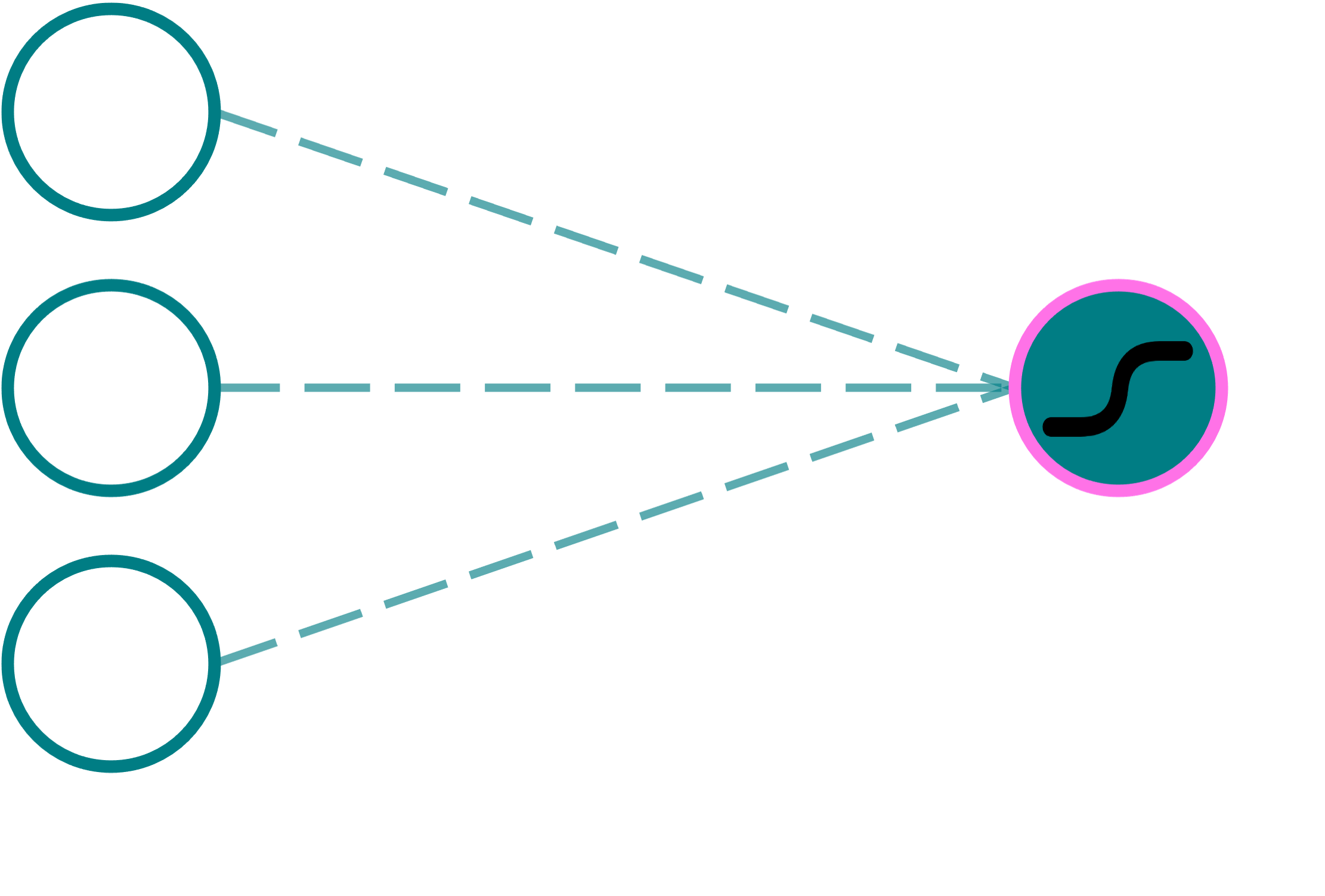
In other words, we may think of each perceptron in a neural network as a smaller model that serves to either make a binary decision based on its inputs (for instance, by producing outputs converging to $0$ or $1$ for the sigmoid activation, outputs converging to $-1$ or $1$ for the $\tanh$ activation), or otherwise extract some useful information from the data (such as using ReLU, which retains $\mathbf{w}\cdot\mathbf{x} + b$ when this quantity is greater than $0$). Each neuron, therefore, is a building block that can be used to model complex patterns in the data by serving as an intermediate feature extractor.
To fully appreciate why this is important, we can look at a simple example. Imagine the four points in the following figure, which are not linearly separable (i.e., a single linear classifier would not be able to separate these points into two classes). However, by using a neural network with a single hidden layer, we can learn a non-linear decision boundary by combining two linear boundaries, such that it separates the two classes.
The figure above shows the XOR problem, which is a classic example of a problem that cannot be solved by a single linear classifier. However, by using a neural network with a single hidden layer, we can learn a non-linear decision boundary that separates the two classes. Before we build such a network, however, think about how you might solve this problem using two linear classifiers instead of one.
To solve the XOR problem by combining two linear classifiers, we can use the fact that the XOR gate is a combination of the AND and the OR gates, combined with a NOT gate, such that $A\ \mathrm{XOR}\ B = (A\ \mathrm{OR}\ B)\ \mathrm{AND}\ \mathrm{NOT}\ (A\ \mathrm{AND}\ B)$. Here, both the OR and AND gates are linear classifiers, and can be represented by a line in 2D space in our example. The NOT gate is a linear classifier as well, but let's put that thought aside for a moment. The figure below shows one possible decision boundary each for the AND and OR gates respectively.
The OR decision boundary labels everything to its right as $1$, and everything to its left as $0$. The AND decision boundary labels everything to its right as $1$, and everything to its left as $0$. The XOR decision boundary, therefore, needs to classify the points that lie to the right of the OR line as $1$, and the points that lie to the right of the AND line as $0$. However, we know from a previous section, that flipping the signs for the weight and bias terms for the AND decision boundary will label the points to its left as $1$ instead. However, we still need to combine these two decision boundaries into a single final prediction.
Let us now finally construct a neural network with a single hidden layer, and think about how it may achieve such a combination. Imagine a neural network, with two input nodes, two nodes in the first hidden layer, and a single output node. Further, we can set the network up in such a way that the top node in the hidden layer represents the OR decision boundary from the above figure, and the bottom node represents the AND decision boundary (whether the direction of prediction is flipped about the line does not actually matter in this setting). How may we do this? Well, we know that the first node should represent a logistic regression that has the same behavior as the OR gate. In other words, its output should be close to $1$ if $A\ \mathrm{OR}\ B$ is $1$, and $0$ otherwise. This, in turn, is nothing but a probability that is based on distance from a line in 2-D space in our example (which is the same OR boundary from our figure). Finally, we know that we can represent a line in two dimensions using a weight vector and a bias term. Therefore, the weights and bias term for the top node in the hidden layer should be such that it represents the OR decision boundary. From the figure above, we can deduce that $\mathbf{w}_1=[1,1], b_1 = -0.5$ produces such a line. Similarly, the weights and bias term for the bottom node in the hidden layer should represent the AND decision boundary, and from our figure we can say that $\mathbf{w}_2 = [1,1], b_2=-1.5$ produces such a line. The final output node should then take the outputs from the two nodes in the hidden layer, and combine them to produce the XOR decision boundary. This setup is shown below:
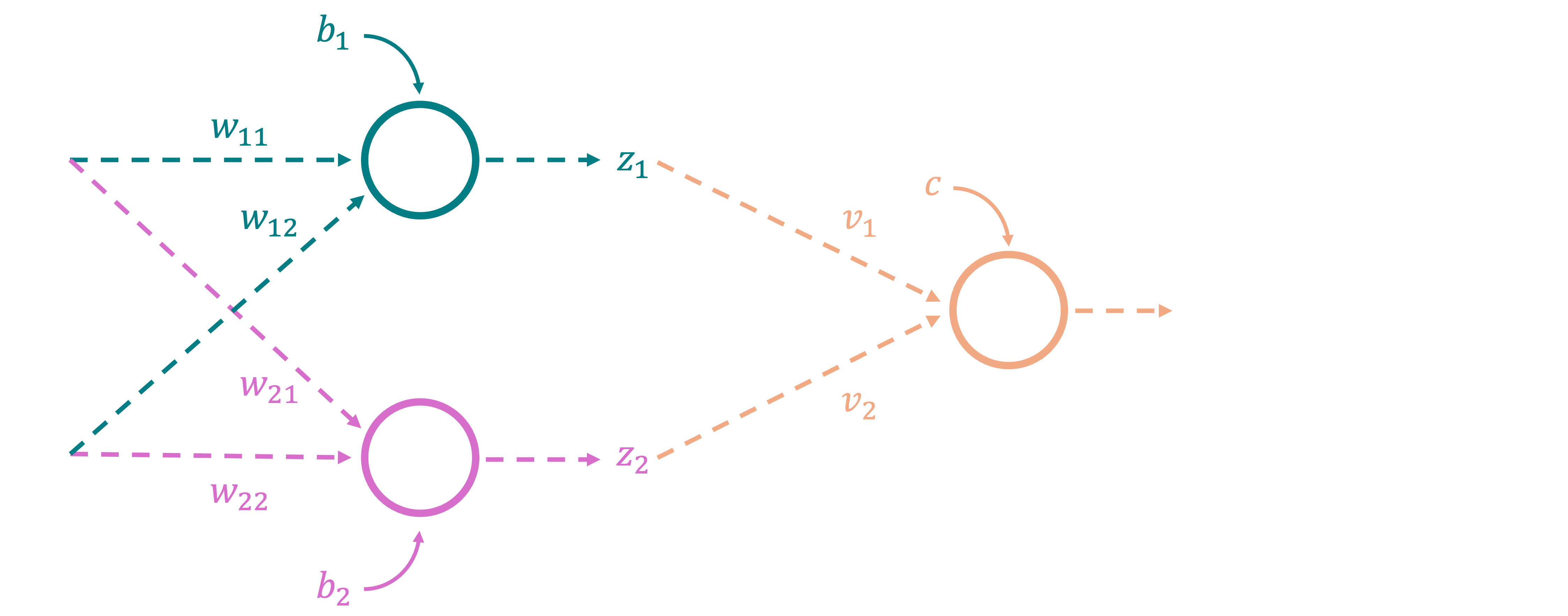
Now, let us work through the network, and see what is actually happening internally. The top node in the hidden layer takes the input $(A,B)$, and produces the value $\sigma(w_{11}x_1 + w_{12}x_2 + b1) = \sigma(\mathbf{w}_1\cdot \mathbf{x} + b1)$. Since we have deliberately set $\mathbf{w}_1 = [1,1], b=-0.5$, we know that the output roughly corresponds to the behavior of the OR gate. For instance, for the point $(0,0)$, we get $z_1 = 1*0 + 1*0 - 0.5 = -0.5$, and $\sigma(-0.5) \approx 0.38$, which is closer to $0$ than it is to $1$. Similarly, for the point $(1,0)$, we get $z_1 = 1*1 + 1*0 - 0.5 = 0.5$, and $\sigma(0.5) \approx 0.62$, which is closer to $1$. The bottom node in the hidden layer takes the same input $(A,B)$, and produces the value $\sigma(w_{21}x_1 + w_{22}x_2 + b2) = \sigma(\mathbf{w}_2\cdot \mathbf{x} + b2)$. Since we have deliberately set $\mathbf{w}_2 = [1,1], b=-1.5$, we know that the output roughly corresponds to the behavior of the AND gate. For instance, for the point $(0,0)$, we get $z_2 = 1*0 + 1*0 - 1.5 = -1.5$, and $\sigma(-1.5) \approx 0.18$, which is closer to $0$ than it is to $1$. Similarly, for the point $(1,1)$, we get $z_2 = 1*1 + 1*1 - 1.5 = 0.5$, and $\sigma(0.5) \approx 0.62$, which is closer to $1$ as expected. Now before we move on to the final output node, let us see what happens when we simply plot the outputs of the two nodes in the hidden layer for all the four points in our original dataset. For instance, for $(0,0)$, the output values are $\mathbf{z} = [0.38, 0.18]$, which forms one point in our new 2-D space. The following figure shows the outputs of the two nodes in the hidden layer for all the four points in the dataset, with the original location of each point denoted in the legend:
Perhaps, the role of the final output node is now becoming clearer. The final output node, in this example, learns its own decision boundary in this latent space, such that it is able to separate the points that lie to the right of the OR line and the left of the AND line as $1$. This is the essence of how a neural network can learn complex patterns in the data by combining simpler decision boundaries learned by individual nodes in the hidden layer! In this new space (above figure), we can draw a linear decision boundary that separates the blue points ($(0,1)$ and $(1,0)$) from the orange points ($(0,0)$ and $(1,1)$), and this line acts as the XOR decision boundary. Specifically, we want the blue points to be classified as $1$ and the orange points to be classified as $0$. The weights and biases for the final output node can be set to $\mathbf{v} = [1,-1], c = -0.22$ to produce such a line, shown below.
The final output node, therefore, takes the outputs of the two nodes in the hidden layer, and produces the value $\hat{y} = \sigma(\mathbf{v}\cdot \mathbf{z} + c)$. For instance, for the point $(0,0)$, we had $z = [0.38, 0.18]$, and thus $\hat{y} = \sigma(1*0.38 - 1*0.18 - 0.22) = \sigma(-0.02) \approx 0.495$. Since this value is closer to $1$ than to $1$, the final prediction for this point is technically correct, although barely so. This is simply down to the fact that we picked the decision boundaries, and therefore, the weights and biases based on intuition, rather than analytically finding the best possible values.
The XOR problem is a classic example of a problem that cannot be solved by a single linear classifier, and requires a non-linear decision boundary. Neural networks, by combining multiple perceptrons in hidden layers, are able to learn such non-linear decision boundaries. The XOR problem is a simple example, but neural networks are capable of learning much more complex patterns in the data, especially when the neural network is deeper and wider. A deeper neural network is one that has more hidden layers, and a wider neural network is one that has more nodes in each hidden layer. Since the neural network acts as a composition of simple linear classifiers using nonlinear activations, a deeper network is able to learn more complex patterns in the data by combining simpler patterns learned by individual layers. One way to think about this is to think of how we can approximate any function using a combination of simple functions, all the way down to approximating curves with straight lines. In the same way, a neural network is able to approximate complex patterns in the data by combining simpler patterns learned by individual layers.
Model Training
Now that we have discussed the theory behind linear classifiers, logistic regression, and neural networks, let us turn our attention to how these models are trained in practice. The process of training a model involves finding the weights and biases that minimize a loss function that captures how badly our model is performing based on our current estimates of its parameters. This is typically done using gradient descent. Think about the XOR problem once again. What is the loss function that we wish to minimize in this case?
Since our network has a single output that lies in the range $[0,1]$, we can interpret the model's output as the probability of the positive class. The loss function that we wish to minimize is, thus, once again the Binary Cross Entropy (BCE) loss, which we've already seen in Logistic Regression. The only difference here, is that the probability of the positive class is given be the output of a neural network, rather than a logistic regression model. For example, for the XOR neural network, the loss is given by $$\mathcal{L}(\mathbf{w}, \mathbf{v}, b, c) = -\sum_{i=1}^{N} y_i \log \sigma(\mathbf{v}\cdot \sigma(\mathbf{w}\cdot \mathbf{x}_i + b) + c) + (1-y_i) \log (1 - \sigma(\mathbf{v}\cdot \sigma(\mathbf{w}\cdot \mathbf{x}_i + b) + c))$$ In general, the BCE loss for a neural network is given by $$\mathcal{L}(\Theta) = -\sum_{i=1}^{N} y_i \log \sigma(f(\mathbf{x}_i; \Theta)) + (1-y_i) \log (1 - \sigma(f(\mathbf{x}_i; \Theta)))$$ where $\Theta$ is the set of all weights and biases in the neural network, and $f(\cdot)$ is the function that computes the output of the neural network. Note that in the general form, we specify the sigmoid function outside of $f(\cdot)$, since the output of the neural network could be anything (such as when using a ReLU activation at the final layer), and we want to map it to the range $[0,1]$ before computing the loss.
The gradient of the loss function with respect to the weights and biases can be computed by applying the chain rule. Modern optimers (such as the ones in PyTorch) do this automatically using a technique called automatic differentiation, where internally, they build a computation graph of the operations that are performed on the input data, and then compute the gradients by traversing this graph backwards. This process is what we discussed in the section on gradient descent. The gradients are then used to update the weights and biases in the direction that minimizes the loss function. This process is repeated for a number of iterations, or until the loss converges. The learning rate is a hyperparameter that controls the size of the steps taken in the direction of the gradients, and is typically set to a small value. The process of training a model also involves splitting the data into a training set and a validation set. The model is trained on the training set, and the performance of the model is evaluated on the validation set. The loss on the validation set is used to tune hyperparameters such as the learning rate, the number of hidden layers, the number of nodes in each hidden layer, and so on. This process is called hyperparameter tuning, and is an important part of training a model. The model is finally evaluated on an unseen test set to get an unbiased estimate of its performance.
Multiclass Classification: So far, we have discussed binary classification tasks, where the output is either $0$ or $1$. However, in many real-world scenarios, we wish to classify data into more than two classes. This is called multiclass classification. One way to extend binary classifiers to multiclass classifiers is to use the one-vs-all strategy. In this strategy, we train a binary classifier for each class, where the class is treated as the positive class, and all other classes are treated as the negative class. The final prediction is then made by selecting the class that has the highest probability according to the binary classifiers. This is a simple and effective strategy, and is used in practice for many multiclass classification tasks. In the context of neural networks, the output layer is simply modified to have as many nodes as there are classes. Each output node may be thought of as an independent binary classifier, classifying each input as either belonging to the $j^{th}$ class, or not. To be precise, this interpretation strictly works only when the activation function at the output layer is the sigmoid function, but in general, any other activations may be thought of as a weighted composition of features used to make the final decision instead.
However, in this form, the outputs of the neural network do not necessarily sum to $1$. To convert the outputs to a valid probability distribution, the output of the network is passed through a softmax function. The softmax function is a generalization of the sigmoid function to multiple classes, and is defined as $$\mathrm{SM}(z)_i = \frac{e^{z_i}}{\sum_{j=1}^{K} e^{z_j}}$$ where $z$ is the output of the neural network, and $K$ is the number of classes. The output of the softmax function is a probability distribution over the classes, and the class with the highest probability is selected as the final prediction. The loss function used in this case is called the Categorical Cross Entropy loss, and is given by $$\mathcal{L}(\Theta) = -\sum_{i=1}^{N} \sum_{j=1}^{K} y_{ij} \log \mathrm{SM}(f(\mathbf{x}_i; \Theta))_j$$ where $y_{ij}$ is the true label of the $i^{th}$ data point for the $j^{th}$ class, and $\mathrm{SM}(f(\mathbf{x}_i; \Theta))_j$ is the predicted probability of the $i^{th}$ data point belonging to the $j^{th}$ class. To further simplify notation, we can use the fact that both the true label and the predicted probability are vectors, and rewrite the loss function as $$\mathcal{L}(\Theta) = -\sum_{i=1}^{N} \mathbf{y}_i \cdot \log \mathrm{SM}(f(\mathbf{x}_i; \Theta))$$ where $\mathbf{y}_i$ is a one-hot encoded representation of the true label of the $i^{th}$ data point, and $\mathrm{SM}(f(\mathbf{x}_i; \Theta))$ is a vector of the same size as $\mathbf{y}_i$, which contains the predicted probabilities of the $i^{th}$ data point belonging to each class.
Convolutional Neural Nets
To understand convolution operations, think about how we can apply a filter to an image. A filter is a small matrix that is applied to an image by sliding it across the image, and performing a dot product between the filter and the portion of the image that it is currently covering. This operation is called a convolution, and is used in convolutional neural networks (CNNs) to extract features from images (or more generally, n-dimensional objects where spatial structure matters). The output of the convolution operation may be interpreted as a feature map, which contains the activations of the filter at each location in the image. By using multiple filters, we can extract multiple features from the image/input, and by stacking multiple convolutional layers, we can learn more complex features from the same input, just like deep feed-forward networks. The operation is best understood through visualization, and the following resources should be helpful:
DeepLizard - Convolutional Neural Nets
CNN Demo
Max Pool Demo
Image Kernels
PyTorch - Conv2d