Search

One of the most fundamental steps towards modeling intelligent behavior is creating systems with the ability to intelligently find solutions. Several real-world problems can often be re-written as a search over their respective state-spaces, which are explicit representations of the possible configurations of the various components of the problem, and how we can move between these configurations by selecting certain actions.

A very natural application for such an approach is its use in finding the best moves in game playing. Imagine, if you will, a game of tic-tac-toe. It is perfectly conceivable that a computer program can enumerate all possible configurations of a 3x3 grid filled with alternating X and O symbols - after all, there are only $255,168$ possible tic-tac-toe boards, not accounting for symmetry or rotation. For modern computers, this number is no longer a limiting factor, given the immense increase in average computational power over the past few decades.

However, game-trees (the state-space representation of a game) that grow exponentially can still be too large for modern computers to enumerate. Consider, for instance, a game of chess, where the number of playable games (note that this is distinct from the number of board configurations) is on the order of $10^{120}$, also known as the Shannon number. To quote the late Prof. Patrick Henry Winston of MIT, "if every single atom in the universe had been running nanosecond-speed calculations since the Big Bang, we still wouldn't have solved a single game of chess." On the other hand, history is witness to Deep Blue, a supercomputer built by IBM, beating the chess Grandmaster Garry Kasparov in 1997. So how did we get there?

Before we can go about writing our own chess engines, we first need to build intuition about how we can represent various problems in terms of searching a state-space, and learn about some techniques to navigate this search-space efficiently.

Interpreting Problems as Search

Route Planning: Consider the problem of navigating the Boston area using the T. We can represent this problem as a search over the state-space of all possible routes between the two stations of interest - the origin and the destination. The actions in this case are the various trains that we can take, and the states are the various stations that we can reach. The cost in this model can be a combination of the monetary cost of the ticket, and time taken. [Here's a time-scale map of the T system.]

In this problem, we are interested in finding the shortest path from origin to destination. We can consider this a search over a graph-representation of the state-space, where each T station is represented as a node, each edge represents a connection between two stations (there may be many edges between two stations), and each edge carries a weight, indicative of the time the connection takes.

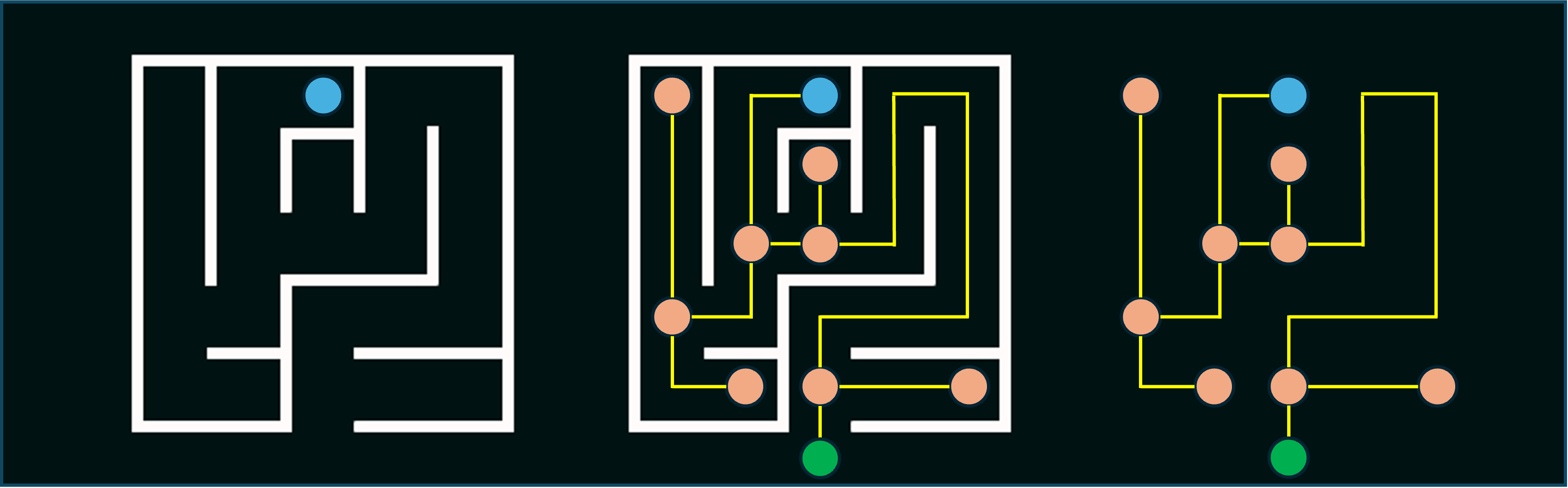
Maze Solving: Similar to route-planning, we can re-imagine a maze as a state-space graph. Each intersection in a maze is represented as a node, with edges originating from this node representing the various directional choices, eventually terminating in neighboring intersections. Here's a quick example:

8-Puzzle: The 8-puzzle is a classic sliding puzzle, consisting of 8 tiles arranged on a 3x3 grid, with one empty square. The tiles are labeled 1-8, and are initially shuffled to a random starting configuration, and the goal is to slide the tiles around to get them back in sorted order. [An online version may be accessed here.] Each configuration of the board can be considered a node in a state-space graph, with edges connecting the neighboring configurations achievable by moving one of the tiles adjacent to the empty square into that position.

Depth First Search

A fundamental approach in graph searching is Depth-First Search (DFS), which explores as far as possible along each branch in a graph until a leaf (node with no outgoing connections to other nodes not seen before) is reached. If the leaf node is not the desired goal state, the search backtracks to the most recent node with an unexplored branch, and continues from there. This process is repeated until the goal state is reached. DFS can be implemented using a stack, which stores the nodes to be explored. Let S be an empty stack (an alternate implementation uses recursive function calls which implicitly uses the call stack instead), let G be the graph, and let s be the start node. DFS, in both variants, is as follows:

function DFS-iterative (G, s):
	S.push( s )
	mark s as visited
	while (S is not empty):
		v  =  S.pop( )
		if v == goal:
			terminate
		for all neighbors w of v:
			if w not visited:
				S.push( w )
				mark w as visited

function DFS-recursive (G, s):
	mark s as visited
	if s == goal:
		terminate
	for all neighbors w of s:
		if w not visited:
			DFS-recursive(G, w)

		

DFS is complete, i.e., if a solution exists, DFS will find it. This stems from the fact that DFS, if run without a termination condition, will eventually visit all nodes in the graph. On the other hand, DFS is not optimal, i.e., it may not necessarily find the shortest path (the best or optimal solution). Since the algorithm explores a selected branch all the way to its leaf node, it is entirely possible that DFS encounters a path to the goal state and terminates, but a subsequent branch that is yet to be explored contains a shorter path to the goal.

This online tool provides an excellent visualization of the algorithm's execution [David Galles, Univ. of San Francisco].
Here is another such tool, with step-wise implementational explanations [Visualgo.net].

Breadth First Search

function BFS (G, s):
	Q.enqueue( s )
	mark s as visited
	while (Q is not empty):
		v  =  Q.dequeue( )
		if v == goal:
			terminate
		for all neighbors w of v:
			if w not visited:
				if w == goal:
					terminate
				Q.enqueue( w )
				mark w as visited

Unlike DFS, BFS is both complete and optimal. Since it visits all nodes at a certain distance from the source node in a given iteration, it is guaranteed to find the shortest path (since any shorter solutions, by design, must have been encountered in a prior iteration). Unterminated, BFS too will visit every node in a connected graph, and thus will find a solution, if one exists.

This online tool provides an excellent visualization of the algorithm's execution [David Galles, Univ. of San Francisco].
Here is another such tool, with step-wise implementational explanations [Visualgo.net].

Iterative Deepening Search

Iterative Deepening Search (IDS) is an algorithm that combines the benefits of both Breadth First Search (BFS) and Depth First Search (DFS) by gradually increasing the depth of the search. IDS is a hybrid algorithm that performs DFS up to a certain depth, then increases the depth limit iteratively until the goal is found. IDS is suitable for scenarios where memory constraints make BFS impractical, and the depth of the solution is unknown.

function IDS (G, s, goal):
	depth_limit = 0
	while (true):
		result = DFS (G, s, goal, depth_limit)
		if result == goal:
			return result
		depth_limit += 1
		
function DFS (G, current, goal, depth_limit):
	S = [(current, 0)] // tuple of (node, depth)
	visited = empty set
	
	while S is not empty:
		v, depth = S.pop()
		
		if v == goal:
			return v
		
		if depth < depth_limit:
			if v not in visited:
				mark v as visited
				for all neighbors w of v:
					if w not in visited:
						S.push(w, depth + 1)
		
	return None

While IDS is slower than BFS due to redundant computations for already covered depths, for graphs with larger branching factors, the difference in runtime is not very significant. For example, if we have a search tree of depth $d$, with a branching factor $b$, the number of redundant computations is: $ (1)b^{d-1} + (2)b^{d-2} + ... + (d)b^{d-d} = \mathcal{O}(b^{d-1})$. The total number of nodes at the bottom level is $\mathcal{O}(b^d)$, which dominates the number of redundant computations, especially for large values of $b$. However, IDS uses the same amount of memory as DFS ($\mathcal{O}(bd)$), compared to BFS's somewhat impractical ($\mathcal{O}(b^d)$).

Uniform Cost Search

Uniform Cost Search extends search to graphs where each edge has a cost. Recall the example of riding the T, with various paths having a different cost based on time taken. The goal is to find the path with the minimum total cost from the start node to the goal node. UCS uses a priority queue to always expand the least costly edge in the process of searching for a path, maintaining a frontier of roughly uniform cost. Upon finding the goal, the algorithm terminates, and is, by design, complete and optimal.

function UCS ( G , s, goal ):
	PQ.push( 0, s, [] )
	while PQ is not empty:
		c, v, path = PQ.pop()
		if v not visited:
			mark v as visited
			path.append(v)
			if v == goal:
				return path
			for all neighbors w of v:
				if w not visited:
					PQ.push( c + WT(v, w), w, path )