Informed Search (Heuristic Search)
So far, our search algorithms were operating based on cumulative cost, but there is no information about whether the chosen paths are getting the agent closer to the goal. Heuristics are functions that estimate or approximate the cost of the cheapest path from the agent's current state to the goal. Informed search algorithms use such heuristics to guide the search towards the goal. Heuristics are most useful when they are either computationally inexpensive (when compared to optimal search), or are readily available as a constant-time lookup.Search Heuristics
Heuristics are essential in situations where finding an optimal solution is computationally expensive or impractical. Instead of exhaustively searching through all possible solutions, heuristics provide a way to prioritize and guide the search toward more promising paths. In some cases, good heuristics lead to an algorithm being optimal, but this is not always the case. Consider the following examples:
- Mazes - Distance to Goal: The distance to the goal is a common heuristic used in maze-solving algorithms. Depending on the problem setup (i.e., limitations on the movement of the agent), one might opt to use straight-line distance (also known as the Euclidean distance). In a grid-world where movement is restricted to horizontal or vertical steps, the Manhattan distance, which is the shortest distance between two points by only moving parallel to one of the axes, is often used. When obstacles are ignored, computing these distances is an $\mathcal{O}(n)$ operation, where $n$ is the number of dimensions in the vector-space where the problem is set. The complexity of the search problem significantly dominates this, thus making this added cost negligible. In maze-solving, $n=2$, and thus calculating the heuristic is essentially a constant time operation. Given the coordinates of the agent ($\mathbf{X}$) and the coordinates of the goal state ($\mathbf{Y}$) where both $\mathbf{X}$ and $\mathbf{Y}$ are vectors in $n$ dimensions,
$$\textrm{Euclidean Distance } = \sqrt {\sum _{i=1}^{n} \left( \mathbf{X}_{i}-\mathbf{Y}_{i}\right)^2 }$$
$$\textrm{Manhattan Distance } = \sum_{i=1}^n |\mathbf{X}_i-\mathbf{Y}_i|$$ - 8-Puzzle - Number of Tiles Out of Place: In the context of the 8-puzzle (a sliding puzzle with 8 numbered tiles and an empty space), the number of tiles out of place may be used as a heuristic that estimates how far the current state is from the goal state. This heuristic is also known as the Hamming distance. Note that this heuristic may not be suited for end-game play, since it does not capture the complexity of getting a given number of tiles that are out of place to their correct positions. Consider for example, the following boards:
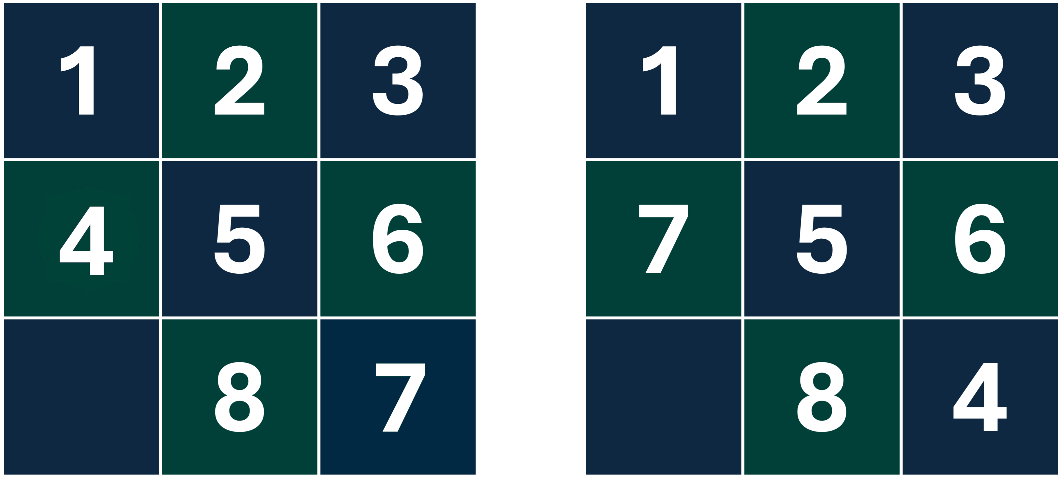
The board on the left only has 1 tile out of place, however, it is an unsolvable configuration, i.e. no sequence of moves can possibly lead to a valid solution. The board on the right is solvable, with 2 pieces out of place, but requires a fairly long sequence of moves to actually solve. - Scheduling - Time to Completion: In scheduling, a potentially useful heuristic might involve estimating the time to completion for each job (based on historical data). Jobs with shorter estimated completion times can then be prioritized, simplifying the scheduling process.
Properties of Heuristics
From the above examples, it is clear that we need a way to evaluate the "goodness" of a heuristic for a given search problem. Fortunately, there are two mathematical properties of heuristic functions that help us establish this.
- Admissibility: Given a state $n$, and a goal state $g$, a heuristic $h(n, g)$ is said to be admissible if it never overestimates the cost of the shortest path between $n$ and $g$. Consider the following graph:
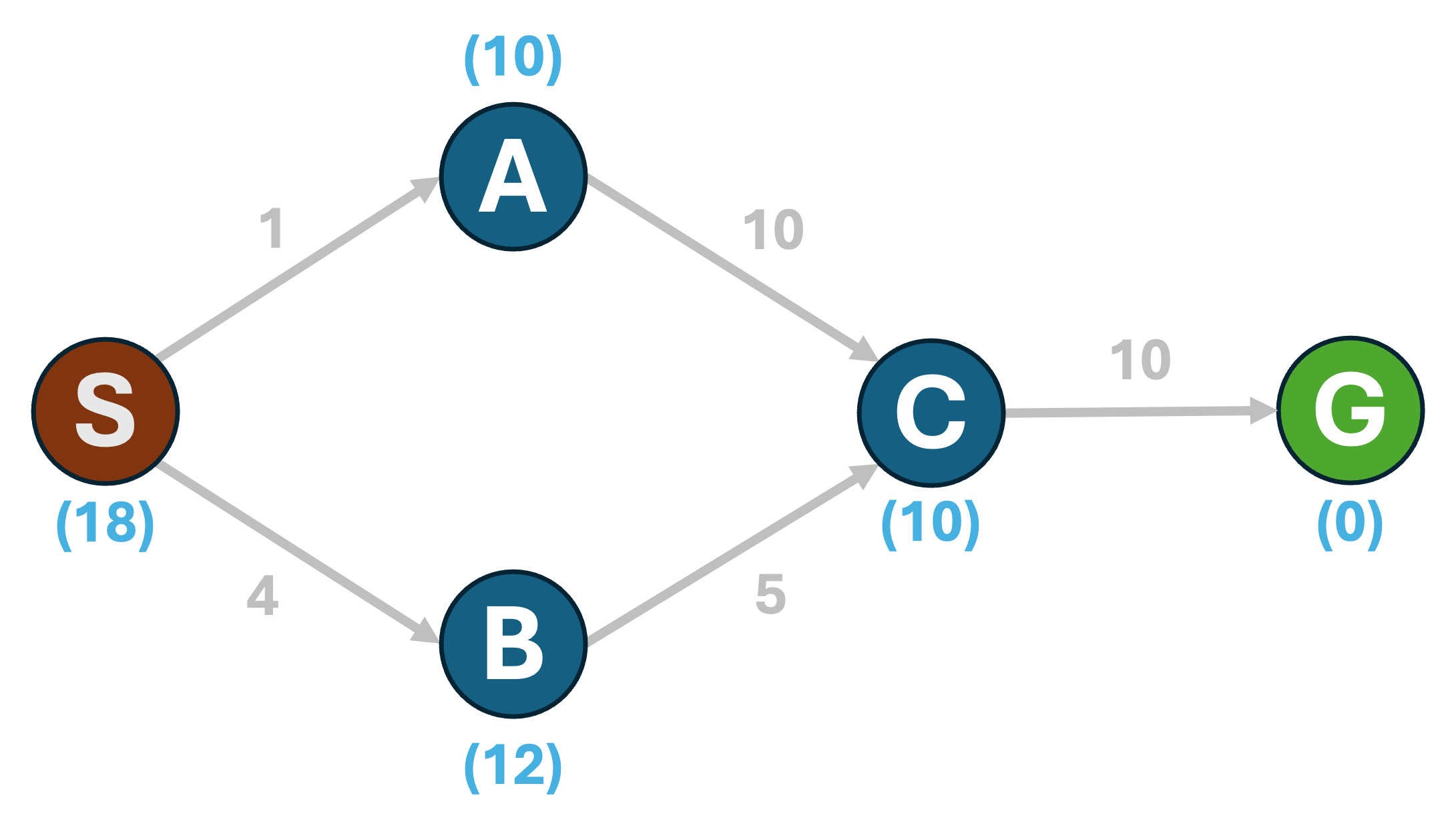 The number within parentheses below each node indicates the heuristic estimate, $h(n)$, of the cost of the shortest path from the node to the goal, G. In this example, we can see that $h(n)$ is always an underestimate of the true shortest-path cost from any node to the goal. E.g., consider the start state, S. The shortest path from S to G is (S,B,C,G) with a cost of 19. The estimate $h(S)=18 \le 19$. If such an inequality holds true for all nodes in the graph, the heuristic is admissible.
Admissibility ensures that we never skip exploring a path that may be optimal - if we allowed a heuristic to overestimate true costs, then the true shortest paths may seem suboptimal to our search algorithm. - Consistency: In the above graph, you may have noticed that in the process of underestimating the shortest-path costs for the sake of admissibility, we have ended up with a rather misleading set of estimates; an agent currently at S would incorrectly believe the path (S,A,C,G) to be the cheapest path. What we are lacking, is monotonicity of estimates as we traverse the graph.
To address this, we turn to consistency. We say that a heuristic $h(n,g)$ is consistent if the heuristic estimate at any given state $n$ is less than or equal to the sum of moving from $n$ to any of its neighbors $n'$, and the heuristic estimate from $n'$, i.e., $h(n)\le c(n\rightarrow n') + h(n')$. Consider the following updated set of heuristic estimates for same graph as before: The estimates we now have are consistent. Under the rules of consistency, the estimate at the current node is a more accurate representation of how the search algorithm should progress. While the search may expand (S,A) first, it will eventually discover that (S,B,C,G) is the cheaper path.
Greedy Best First Search
Now that we have learnt how to evaluate heuristics, we can use them to guide our search algorithms. Greedy best first search is a simple algorithm that uses only the heuristic to prioritize the exploration of nodes, not taking actual traversal cost into account. The algorithm is as follows.function GBFS ( G , s, h, goal ):
PQ.push( h(s,goal), s, [] )
while PQ is not empty:
c, v, path = PQ.pop()
if v not visited:
mark v as visited
path.append(v)
if v == goal:
return path
for all neighbors w of v:
if w not visited:
PQ.push( h(w,goal), w, path )A* Search
A Star search is a one example from the class of best-first search algorithms, which, given a consistent heuristic is both complete and optimal. A* search chooses nodes on the basis of a function $f(n)$ which combines the cumulative cost (of moving from start to $n$) and the heuristic estimate of how far the goal is from the node $n$. The algorithm proceeds similarly to UCS, by maintaining a frontier of roughly equal costs, and expanding the node with the lowest $f(n)$ value. The key difference between UCS and A* is that in UCS, $f(n) = g(n)$, where $g(n)$ is the cumulative cost to get to node $n$, whereas in the case of A*, $f(n) = g(n) + h(n)$, where $h(n)$ is the heuristic estimate. The algorithm is as follows.function ASTAR (G, s, goal):
PQ.push( H(s, goal), 0, s, [] )
while PQ is not empty:
h, c, v, path = PQ.pop()
if v not visited:
mark v as visited
path.append(v)
if v == goal:
return path
for all neighbors w of v:
g = c + WT(v, w)
PQ.push( g + H(w, goal), g, w, path )Walkthrough: Consider the graph below, with values along the edges representing the cost of the edge, and the values in parentheses below each node representing the heuristic estimate $h(n)$.
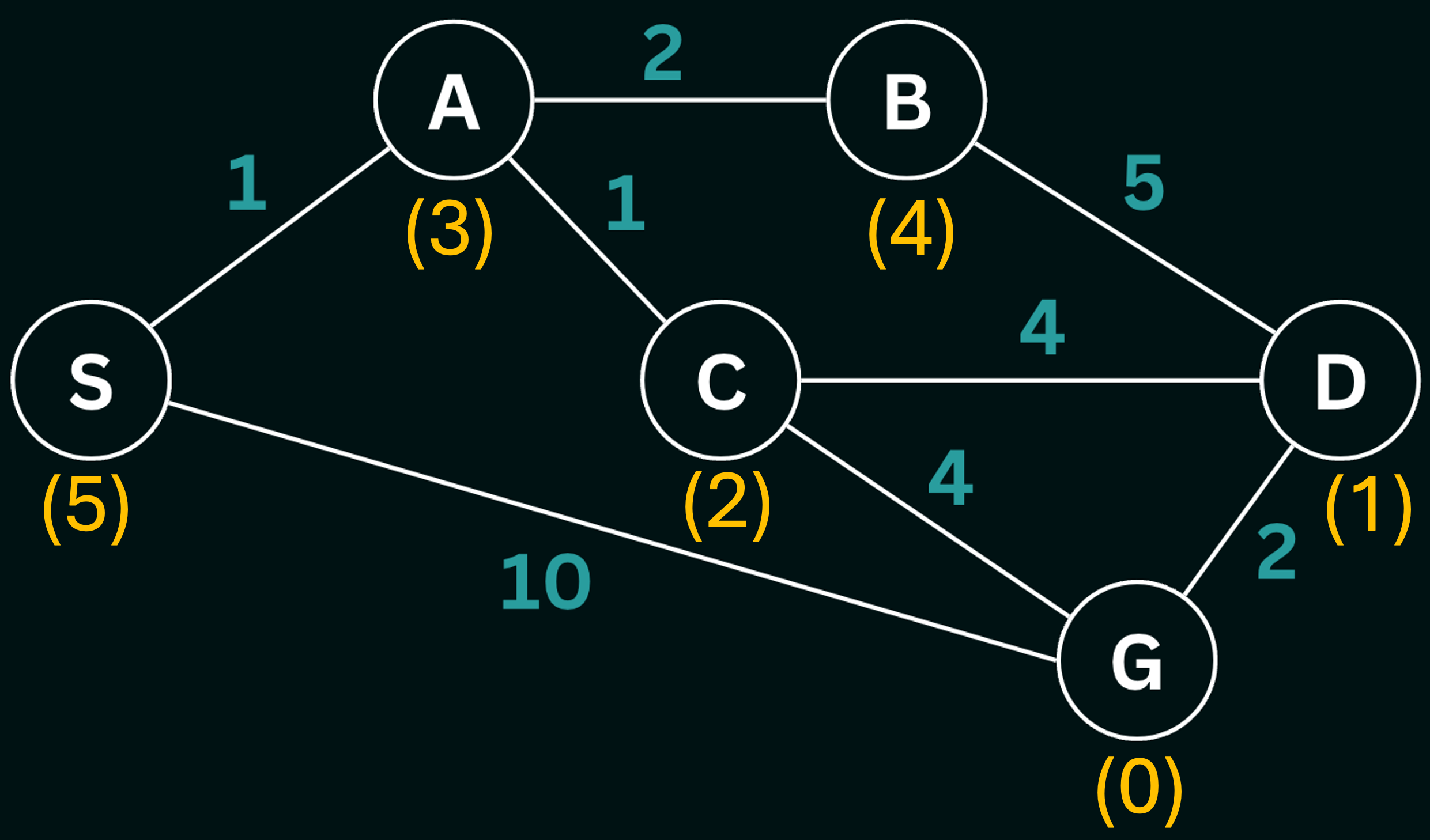
At $S$ we have two possible paths, $S->A$ or $S->G$. Let’s evaluate these paths:
$S$ → $A$
$f(A)=g(A)+h(A)$
$f(A)=1+3$
$= 4$
$S$ → $G$
$f(G)=g(G)+h(G)$
$f(G)=10+0$
$= 10$
Since, $f(A) < f(G)$ we add the node $A$ to the $frontier$. At $A$ we have two paths at our disposal, $S->A->B$ or $S->A->C$. Let’s evaluate these paths:
$S$ → $A$ → $C$
$f(C)=g(C)+h(C)$
$f(C)=(1+1)+2$
$= 4$
$S$ → $A$ → $B$
$f(B)=g(B)+h(B)$
$f(B)=(1+2)+4$
$= 7$
Since, $f(C) < f(B)$ we add the node $C$ to the $frontier$. At $C$ we have two paths at our disposal, $S->A->C->D$ or $S->A->C->G$. Let’s evaluate these paths:
$S$ → $A$ → $C$ → $D$
$f(D)=g(D)+h(D)$
$f(D)=(1+1+4)+1$
$= 7$
$S$ → $A$ → $C$ → $G$
$f(G)=g(G)+h(G)$
$f(G)=(1+1+4)+0$
$= 6$
Since, $f(G) < f(D)$ we add the node $G$ to the $frontier$. In the loop following this addition, we pop the node $G$ and undergo a goal test and eventually break out of the loop. Note that the heuristic in this example is consistent, and therefore lets A* search find the optimal path.
Beam Search
Beam search is a heuristic search algorithm which seeks to address the memory complexity of A* search. It does so by focusing on the nodes with the best heuristic within a limited set, and expanding only the $\beta$ best nodes at each level.
Beam Search utilizes a breadth-first style approach, and it generates all successors of the current state, but expands only a specified number, $\beta$, of states based on their heuristic cost. The parameter $\beta$ is known as the beam width. If $b$ represents the branching factor (assuming that the branching factor is constant for simplicity), the number of nodes under consideration at every depth is $\beta \times b$, where $\beta\in [0,1]$. Reducing the beam width results in the pruning of more states. The variation of $\beta$ alters the approach of the algorithm - when it is set to $1/b$, the algorithm emulates a hill-climbing search, where a singular best node is consistently chosen from the successor nodes. On the other hand, $\beta = 1$ corresponds to a standard A* search, where all nodes are selected for expansion.
Employing a beam width serves to bound the memory requirements by limiting the number of sub-trees that are to be explored. However, this comes at the expense of completeness and optimality, as there is a risk that the best solution may not be found. There is always a possibility of pruning branches containing the goal state entirely, which makes finding any solution (and as a result, the optimal solution) impossible.
The beam search algorithm follows the A* search algorithm closely with a few minor changes:
function BEAM-SEARCH (G, s, goal, beam_width):
    PQ.push(H(s, goal), 0, s, [])
    while PQ is not empty:
        h, c, v, path = PQ.get()
        if v not visited:
            mark v as visited
            path.append(v)
            if v == goal
                return path
            neighbors = get_neighbors(G, v)
            for w in beam_select_neighbors(neighbors, beam_width):
                g = c + WT(v, w)
                PQ.push( g + H(w, goal), g, w, path )