Local Search

The preceding discussions on search algorithms delved into methods for traversing state-space graphs from an initial state to a goal, emphasizing the construction and the preservation of a path throughout the process. However, many real-life problems do not focus on the specific path taken to reach the goal. Examples of such problems include job-shop scheduling, automatic programming, telecommunications network optimization, vehicle routing, and portfolio management. In these cases, the focus is primarily on the final configuration of the solution, rather than the journey taken to attain it.

With this in mind, we now turn our attention to local search methods. Unlike their counterparts, local searches operate exclusively on the current node, often choosing to evaluate its immediate neighbors without retaining any path in memory. Local search algorithms offer two key advantages in scenarios where the path to the goal is inconsequential:

• Lower memory requirements : since they only operate on a singular node and are not retaining paths while progressing through the state space, these algorithms usually have a constant space complexity.


• Continuous states : they can find reasonable solutions in infinite state spaces which classical search algorithms are not well-suited to. Local searches achieve this by moving in small steps towards a specific direction to either maximize or minimize an objective in a continuous space.

Thanks to these advantages, local searches prove particularly useful for optimization problems. Typically, these problems feature a continuous state-space landscape characterized by both a location and an elevation, represented by a heuristic or a cost function specific to the problem.

Hill Climbing

Hill-climbing is a type of local search algorithm. Hill climbing iteratively moves in either an increasing/ascent or decreasing/descent direction based on the problem objective. The algorithm terminates when it reaches a "peak" in case of a maximization problem, i.e., no neighbor has a higher objective function value, or a "valley," when the neighbor has no lower value in case of a minimization problem. Hill-climbing can be summarized with the following general structure:

function HILL-CLIMBING(G, s, goal):
    current = s
    while True:
        neighbors = get_neighbors(G, current)
        best_neighbor = None
        best_value = calculate_value(current) 
        for neighbor in neighbors:
            neighbor_value = calculate_value(neighbor)
            if neighbor_value > best_value: 
                best_neighbor = neighbor
                best_value = neighbor_value
        if best_neighbor is None or best_value <= calculate_value(current):
            return current
        current = best_neighbor

This particular approach is one of several related variants of hill-climbing, and is called Steepest-Ascent Hill Climbing. Here, we iterate over all neighbors to pick the best one at each step. In contrast, another commonly seen implementation is to generate a neighboring state, and simply accept it if the score is better than the current state, rather than iterating over all neighbors to find the best one. This latter approach is known as First-Choice Hill Climbing.

Local Optima

Hill-climbing approaches, while often effective, may fail to produce an optimal solution in certain instances. This may happen as a result of the search getting stuck in a local optimum. This can be thought of as exploring the "landscape" of an objective function in an $n$-dimensional vector space. The objective function's landscape may have several points of inflection, causing the search to get trapped in a "valley" (local minimum) or a "peak" (local maximum). Since our local search only moves in one direction, it may completely miss better solutions (deeper valleys or taller peaks) as a result of this.

Ridges: Ridges are sequences of local optima. The presence of multiple local optima makes it challenging for the algorithm to navigate and converge towards a global optimum, as it may become trapped in one of the multiple vicinities.

Plateaus: A plateau refers to a flat area in the state-space landscape, which can be a flat local optimum or a shoulder from which some future progress is posible. Plateaus pose challenges for hill-climbing algorithms as there might be cases where no successor value is available for the algorithm to choose from, resulting in being stranded without further progress.

Dealing with Local Optima: Here, we discuss two commonly used strategies for dealing with local optima. To motivate both strategies, consider the following objective function ($g(w)=\sin(3w)+0.1w\ +\ 0.3$), plotted below.


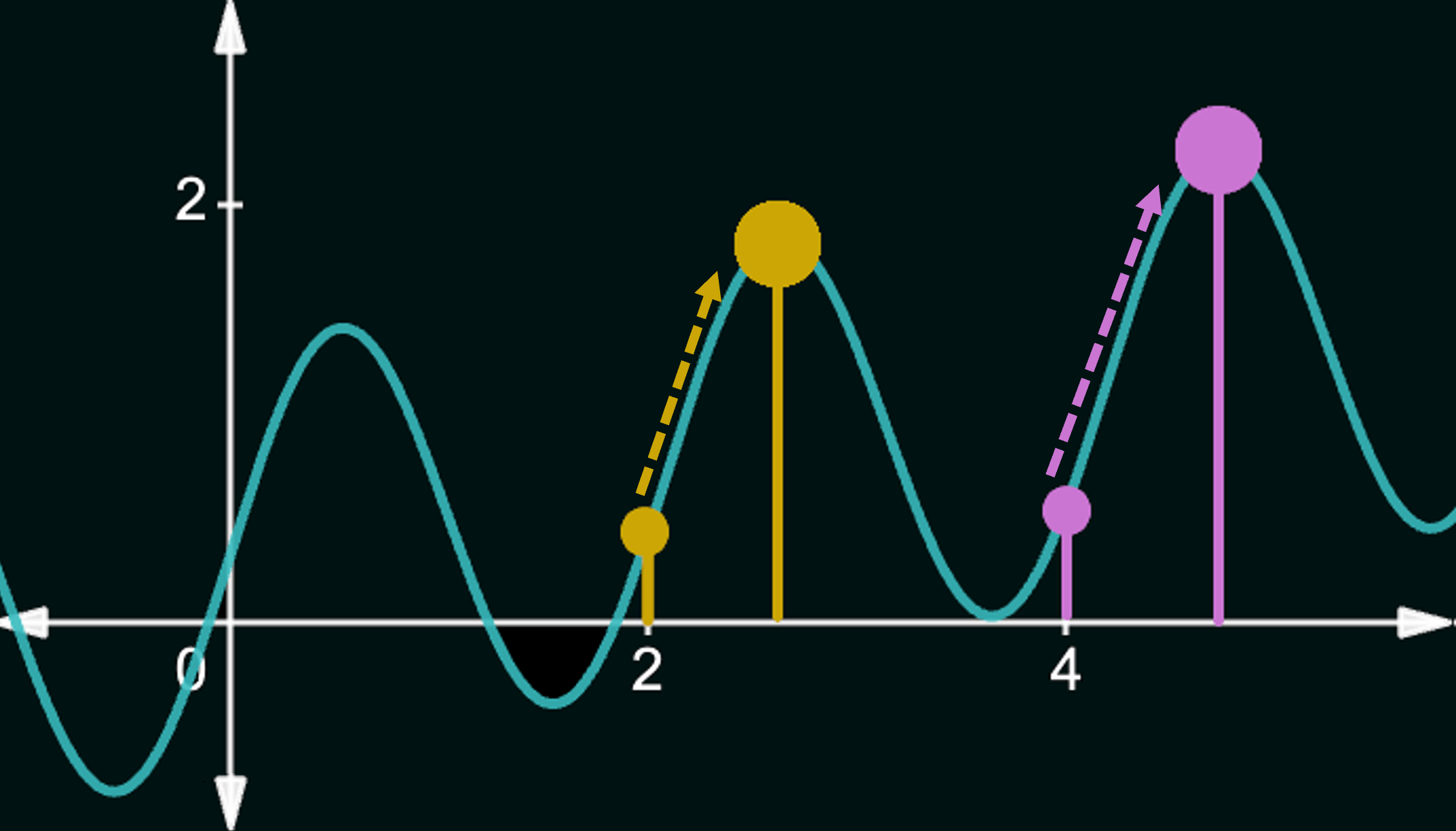
If we start at $x=2$ and attempt to maximize our objective, then hill-climbing leads us to the local maximum at $x\approx 2.6$, whereas the global maximum lies at $x\approx 4.6$. This is a result of the algorithm being stuck in a local optimum. However, if we had either started at $x=4$, or had somehow been able to move from the local optimum to $x=4$, then we could have subsequently reached the global maximum.

Random Restarts: One of the most popular methods to circumvent getting stuck in local optima is to randomly restart the hill-climbing process with a different initial state. In the above example, if the first run started at $x=2$, then a random restart could, in theory, get us to start from, say, $x=4$ (really any value on either slope of the optimal peak), which would lead us to the global optimum.

Random Downhill Steps: A second way to wiggle our way out of local optima is to allow steps that lead to a worse objective function value with a small probability. In the above example, from the local optimum peak around $x=2.6$, if we allowed the search algorithm to accept a neighbor on its right (combined with the step-size being large enough), then a subsequent step could get us to the global optimum. This approach is also known as Stochastic Hill Climbing.

Simulated Annealing

Simulated Annealing can be thought of as an extension to stochastic hill-climbing discussed above. Simulated Annealing draws inspiration from metallurgical processes, where metals are heated to a high temperature and then gradually cooled to remove defects and optimize their crystal structure. Similar to this physical process, the algorithm accepts a worse solution with a probability that decreases over time - encouraging an initial exploration stage, where solutions with a much worse energy or score have a significantly higher probability of being accepted. This allows the algorithm to escape local optima and explore other regions of the search space.

Mathematically, the idea is fairly simple. We assume an initial temperature, $T$ that exponentially decays over time, simulating the rapid cooling of hot metal. This is achieved simply by multiplying the temperature $T$ with a constant $d\in [0,1]$ after every iteration. The objective function (called the Energy function in this setting) value is conceptually similar to hill-climbing, and quantifies how good a solution is, with the notable exception that Simulated Annealing generally seeks to solve minimization problems, i.e., we aim to lower the energy of our solution. Implementationally, this simply means that a better solution is one that has a lower energy value.

The algorithm can be summarized as follows:

function SIMULATED-ANNEALING(G, s, goal, T, d):
	current = s
	best = s
	while True:
	    neighbor = generate_neighbor(G, current)
	    if Energy(neighbor) <= Energy(current):
	        current = neighbor
	        best = neighbor
	    else:
	        if random(0,1) <= e^((Energy(current)-Energy(neighbor))/T):
	            current = neighbor
	        else:
	            continue
	    T = T * d
	if converged:
	    return best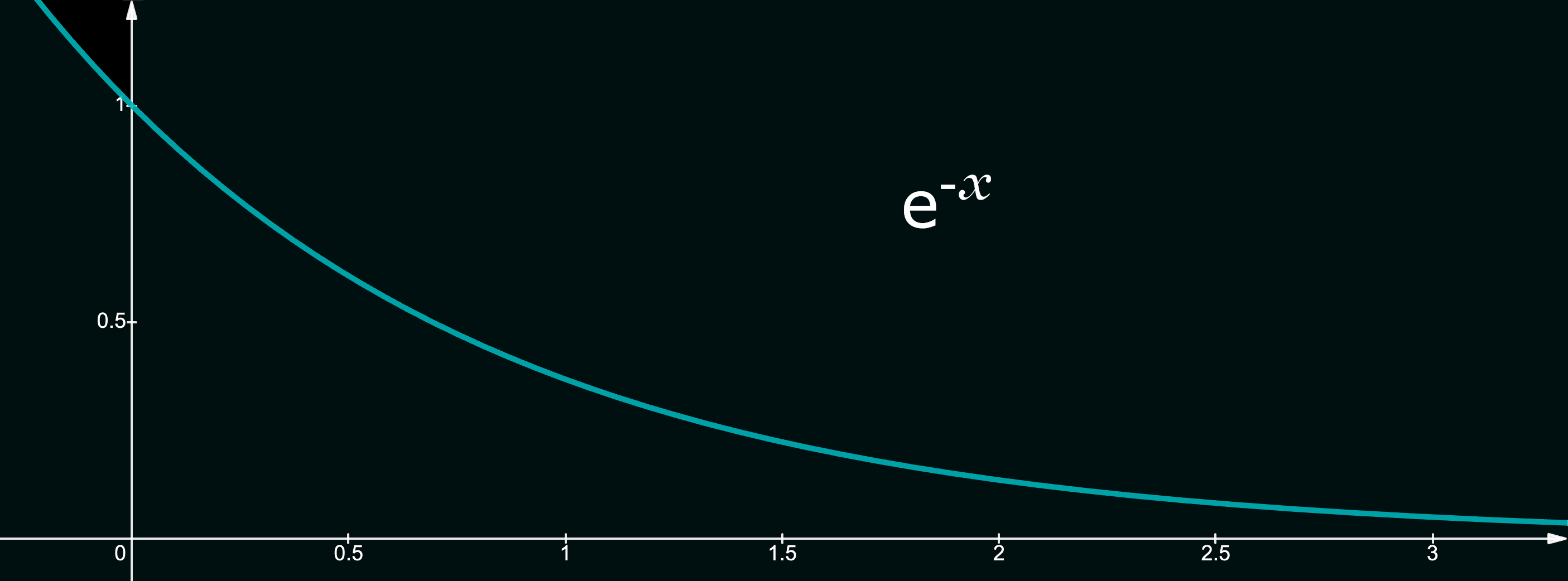

At each iteration, the algorithm accepts the newly generated neighbor if its energy is lower than the current state, and accepts it with a probability of $\mathrm{e}^{(\textrm{Energy(current)-Energy(neighbor)})/T}$ if the energy is higher, where $\mathrm{e}$ is Euler's number. The probability of accepting a worse solution decreases exponentially as the temperature $T$ decreases. Here's some insight into how this works. First, note that we only need to compute this probability when the energy of the generated neighbor is higher than the energy of our current solution. Therefore, the numerator in the exponent, i.e. $\textrm{Energy(current)-Energy(neighbor)}$, is always negative giving us a function of the form $f(x) = \mathrm{e}^{-x}$. Now the exponent is inversely proportional to the temperature $T$, and thus as the temperature decreases, the absolute value of the exponent increases. Essentially, we're now looking at the behaviour of the function $f(x) = \mathrm{e}^{-x}, x \ge 0$, plotted below. You can observe that for a high temperature, the resulting probability of accepting a worse solution is close to one, but as the temperature $T$ decreases, this probability decreases exponentially.

Local Beam Search

Local Beam Search is, put simply, a parallel implementation of hill climbing and its variants, where we maintain a set of $k$ states at each iteration. The algorithm starts by generating $k$ initial solutions, and then proceeds by generating successors for all states in this current set using any hill climbing approach. The algorithm then selecting the $k$ overall best solutions from the resulting set (consisting of current solutions and their successors), in practice, behaving like $k$ separate searches that inform each other by pooling their solutions at the end of each iteration. The algorithm terminates when a goal state is reached or when a specified number of iterations have been completed.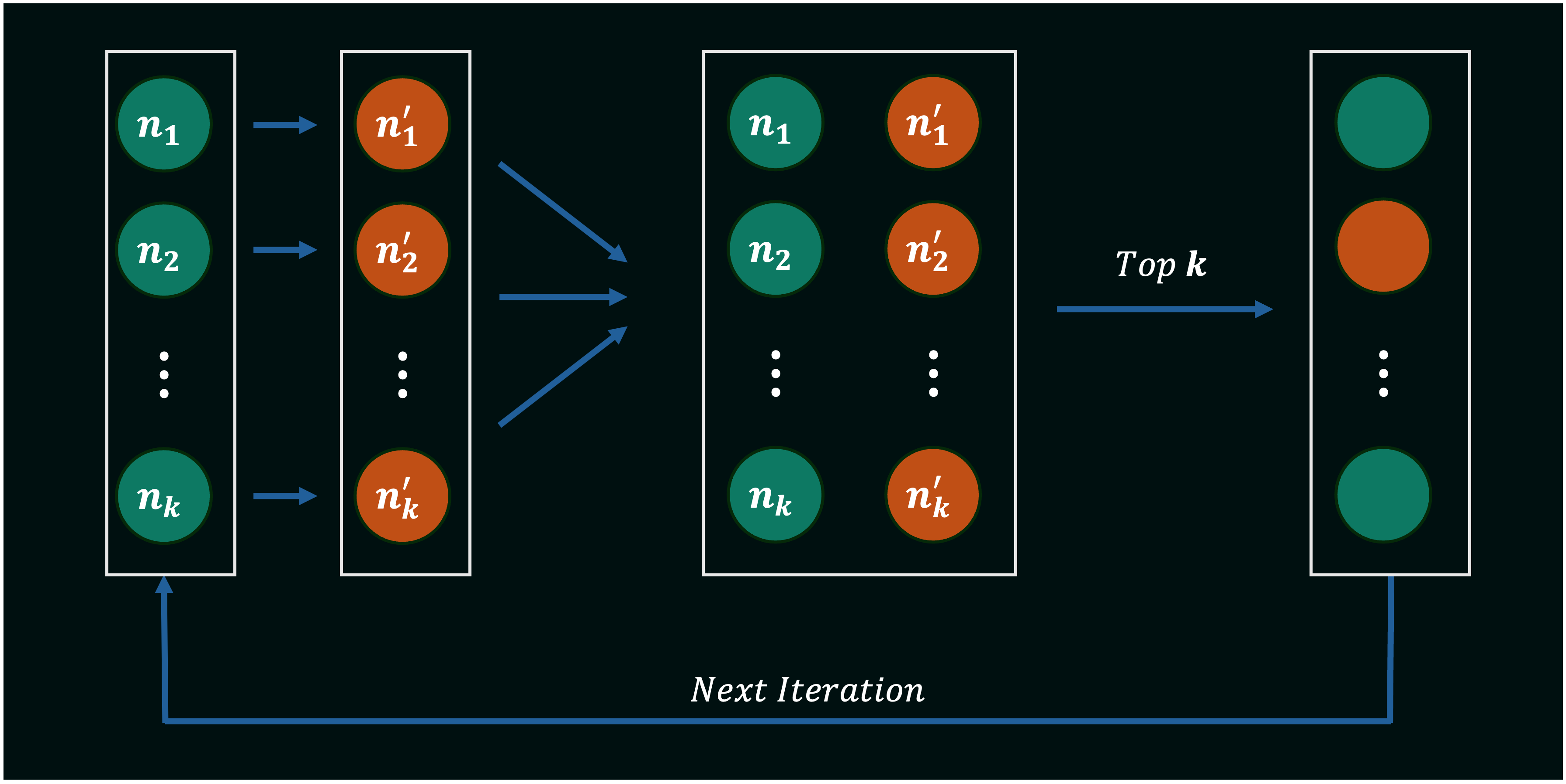

Genetic Algorithms

Genetic Algorithms are a class of search algorithms inspired by the process of natural selection, and can be viewed as an extension/combination of some of the local search techniques we have discussed so far. The algorithm, much like local beam search, maintains a population of candidate solutions, and iteratively applies genetic operators to the population to generate new candidate solutions. These genetic operators broadly consist of mutations and crossovers, discussed below. The algorithm proceeds by iteratively generating new candidates using these operators, and then using a fitness function to retain some subset of the best-performing solutions, in a workflow similar to local beam search.

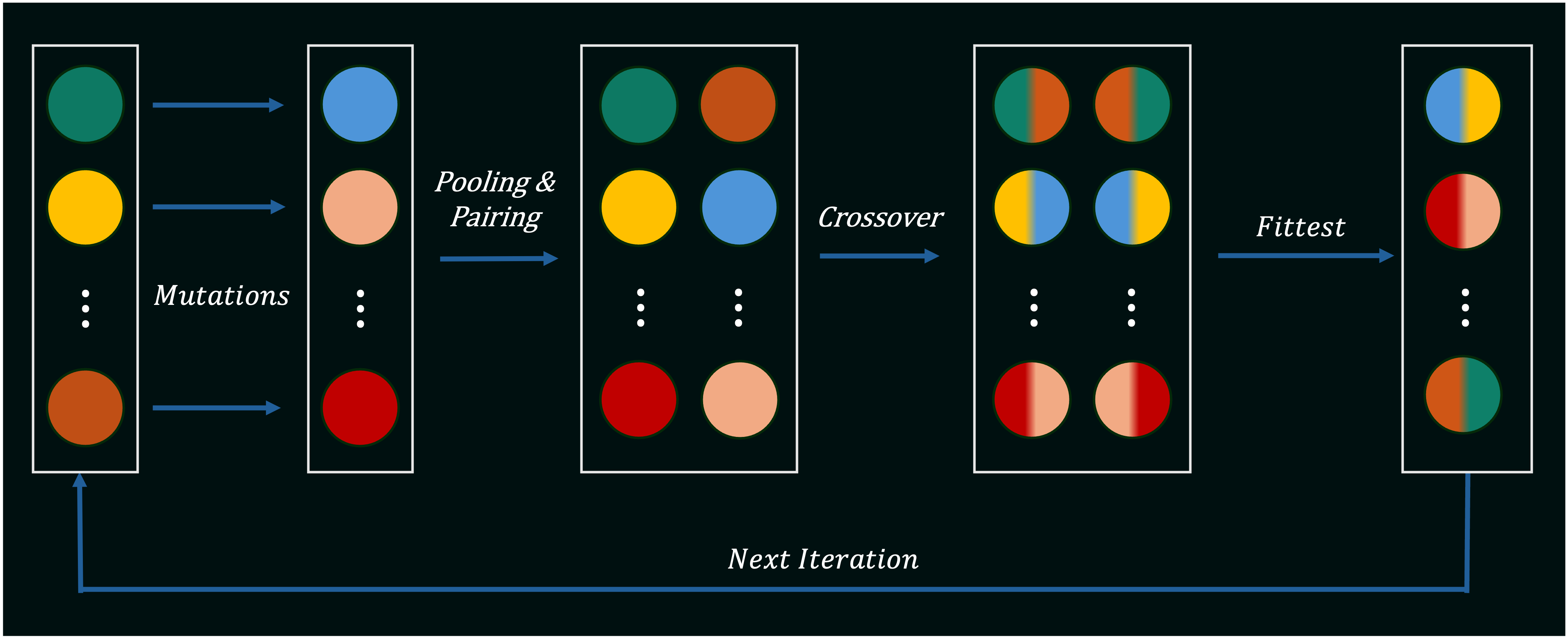
Mutations: These are random changes to a candidate solution, just like in regular hill climbing. For example, in the case of a binary string, a mutation could involve flipping a single bit from 0 to 1 or vice-versa. In the case of a real-valued vector, a mutation could involve adding a small random number to one of the vector's elements. In the case of the traveling salesman problem, a 2-opt swap could be a mutation. Mutations are used to introduce new information into the population, and to prevent the algorithm from getting stuck in local optima. The rate at which these random changes are applied to each candidate solution is controlled by a parameter called the mutation rate, and may vary throughout the execution of the program (similar to how we decrease probability of large changes over time in Simulated Annealing).

Crossovers: These are operations that combine two candidate solutions to produce one or more new candidate solutions. For example, in the case of a binary string or a real-valued 1-dimensional vector, one possible crossover could involve taking the first half of one parent and the second half of another parent to produce a new child string/vector. In the case of the traveling salesman problem, crossovers might involve more steps and some logical parsing of the two parent solutions (see below). Crossovers are used to combine information from two candidate solutions that are already good, in the hopes of producing an even better solution.

Complex crossovers may often be necessary, especially in cases where the validity of a solution depends on the structure of its representation. For example, consider the traveling salesman problem with 5 cities, named A, B, C, D and E. Assuming all cities are connected, one possible solution could be the string "ABCDEA", which represents the order in which the cities are visited. A second candidate solution could be AECDBA. Now, let's try and combine these solutions using a crossover operation. A simple crossover between the two parents "ABCDEA" and "AECDBA" where we combine the first half of the first parent with the second half of the second parent would yield the string "ABCDBA", which is not a valid solution to the TSP. This is because the child visits city B twice, and does not visit city E at all. A more complex crossover could involve parsing the two parents and combining them in a way that ensures that the child visits each city exactly once. This is known as the Order Crossover (OX) operator. For further reading on genetic operations, please refer to these notes by Dr. Lluís Alsedà, Universitat Autònoma de Barcelona.