Games & Adversarial Search

In multi-agent environments, each agent needs to account for the actions taken by other agents in the environment, and their impact on its own objective. In competitive multiagent environments, agents have conflicting goals, and the best outcome for all players involved is usually a compromise. In adversarial search - a subset of search problems - we first model a basic two-player game by treating the environment as a deterministic, fully-observable, turn-based, zero-sum game. In zero-sum games, one player's win or gain is another player's loss, resulting in a net zero change in the total 'wealth', or points.

Minimax

Consider a turn-based game featuring two players - MAX and MIN. MAX starts by playing the first move, after which the game unfolds in an alternating sequence until reaching a terminal state. Like many real-world games, points are awarded to the winner which are equivalently considered penalties for the loser; in our scope, we assume that this game is zero-sum. Specifically, we now assume that each terminal state of this game is assigned a single numerical score/value, which we will call the $\texttt{RESULT}$ of the end-state for the game. Since the players have opposing objectives, we assume that MAX always wants to steer the game towards the largest possible $\texttt{RESULT}$, whereas MIN always tries to minimize this score. In other words, $\texttt{RESULT}$ captures MAX's objective, and the negative of MIN's objective.

As opposed to traditional search problems where the focus is on finding an optimal sequence of actions leading to the goal, the goal of adversarial search is to reason about how the game unfolds, accounting for the fact that two players with opposing objectives are both playing optimally at all times. This look-ahead enables each player to make a move that is either globally optimal (if the search tree spans the entire game), or locally optimal (optimal when only looking at the next $k$ moves, may not be best overall move). This game is set up as follows: the current player at a particular state is $s$ denoted by $\texttt{PLAYERS}(s)$, and $\texttt{UTILITY}(s, p)$ is an objective function providing the value of the game (think of this as the utility for the player) from a state $s$ for player $p$. Consider the following game-tree, where both players have 3 action choices, MAX plays first and the game ends after both players take one turn each. [Example taken from AIMA 4th Ed: Ch. 5]

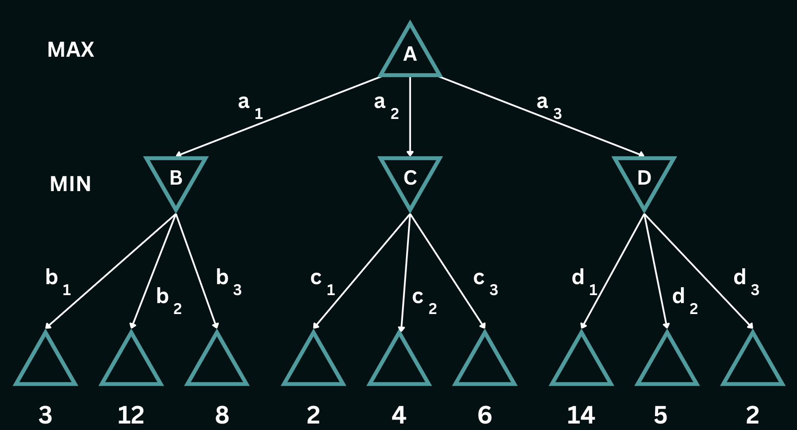
In the above game-tree, $a_1$, $a_2$ and $a_3$ are the possible moves that MAX can choose to play. In response to $a_1$, MIN can play $b_1$, $b_2$ or $b_3$, in response to $a_2$, MIN can play $c_1$, $c_2$ or $c_3$ and so on. The possible end-game utilities for this tree are the numeric values shown below the terminal states, ranging from $2$ to $14$. Given such a tree, the optimal contingent strategy that the current player can take is determined by the **minimax value** of the node, which we denote as $\texttt{MINIMAX}(n)$. The minimax value of a node is the utility of being in the corresponding state, *assuming that both players play optimally* from that node to the end of the game. MAX prefers to move to a state of maximum value, whereas MIN prefers a state of minimum value. So we have the following cases:

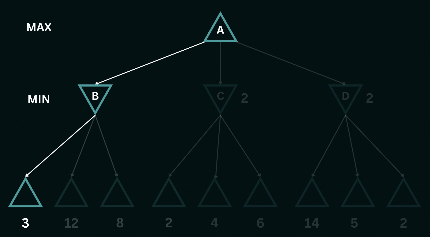
$\texttt{MINIMAX}(s)=\begin{cases} \texttt{UTILITY}(s)\; \textrm{if s is terminal}\\ \max_{a \in Actions(s)} \texttt{MINIMAX}(\texttt{RESULT}(s))\; \mathrm{if\ \texttt{PLAYER}(s)=\texttt{MAX}}\\ \min_{a \in Actions(s)} \texttt{MINIMAX}(\texttt{RESULT}(s))\; \mathrm{if\ \texttt{PLAYER}(s)=\texttt{MIN}}\end{cases}$

In the given game tree, At $B$, $\texttt{MINIMAX}(B)$ would be $3$, At $C$, $\texttt{MINIMAX}(C)$ would be $2$ and at $D$, $\texttt{MINIMAX}(D)$ would be $2$, assuming that the $\texttt{MIN}$ plays optimally. $\texttt{MAX}$ would then play $a_1$ with a utility of $3$ since this is the maximum utility the player can possibly obtain, given that paths to higher utility would never be chosen by $\texttt{MIN}$. The solved tree (the optimal game) would be as follows:

We now discuss the general structure of the MINIMAX algorithm, that seeks to evaluate optimal gameplay with some look-ahead, accounting for an adversary's actions. The algorithm is recursive, and is called on the root node of the game tree. The algorithm is recursive, and can be summarized as follows:

function MINIMAX(node, depth, player):

	if depth = 0 or node is terminal:
		return UTILITY(node)

	if player == MAX:
		U = []
		for every child of node:
			U.append(MINIMAX(child, depth - 1, MIN))
		return max(U)

	else:
		U = []
		for every child of node:
			U.append(MINIMAX(child, depth - 1, MAX))
		return min(U)
					

The algorithm explores the search tree in a depth-first fashion. Applying this algorithm to the example above using a depth of 2, the process begins by descending through the leftmost branch, all the way down to the leaves. The $\texttt{UTILITY}$ function evaluated at the leaves gives us the values $3$, $12$, and $8$, respectively. These are the outcomes, or the heuristic utility values of the terminal states. The algorithm then determines the minimum of these values, which is $3$, and assigns it as the backed-up value for node $B$. A similar procedure yields values of $2$ for nodes $C$ and $D$. Finally, the algorithm ascends to the root node, where it computes the maximum of the backed-up values for nodes B, C, and D, resulting in choosing the state which returns a backed-up value of $3$. If the maximum depth of the tree is $d$ and there are $b$ legal moves at each point, then the time complexity of the minimax algorithm is $\mathcal{O}(b^d)$ while the space complexity is $\mathcal{O}(bd)$.

Alpha-Beta Pruning

Minimax search is a powerful algorithm used in decision-making within competitive environments. In practice, however, it is limited by the exponential growth in the number of game states that are generated as the tree's depth increases. The $\texttt{MINIMAX}$ algorithm explores and expands all nodes and subtrees of the game tree, leading to a high time complexity. To address this issue, we explore a technique called alpha–beta pruning, where the key idea is to eliminate the unnecessary exploration of subtrees that are known to be suboptimal. While this does not eliminate the inherent exponential time complexity, alpha–beta pruning allows us to reduce the time complexity to the square root of that of $\texttt{MINIMAX}$ on average. This can also be interpreted as using the same number of computations as MINIMIAX to explore twice the depth in the search tree.

The alpha-beta pruning algorithm is a modification of the $\texttt{MINIMAX}$ algorithm, where we introduce two new parameters, $\alpha$ and $\beta$, that keep track of the best value that the maximizing player can obtain and the best value that the minimizing player can obtain, respectively. The algorithm is recursive, and can be summarized as follows:

function ALPHA-BETA(node, depth, alpha, beta, player):

	if depth = 0 or node is terminal:
		return UTILITY(node)

	if player == MAX:
		for every child of node:
			alpha = max(alpha, ALPHA-BETA(child, depth - 1, alpha, beta, MIN))
			if beta <= alpha:
				break
		return alpha

	else:
		for every child of node:
			beta = min(beta, ALPHA-BETA(child, depth - 1, alpha, beta, MAX))
			if beta >= alpha:
				break
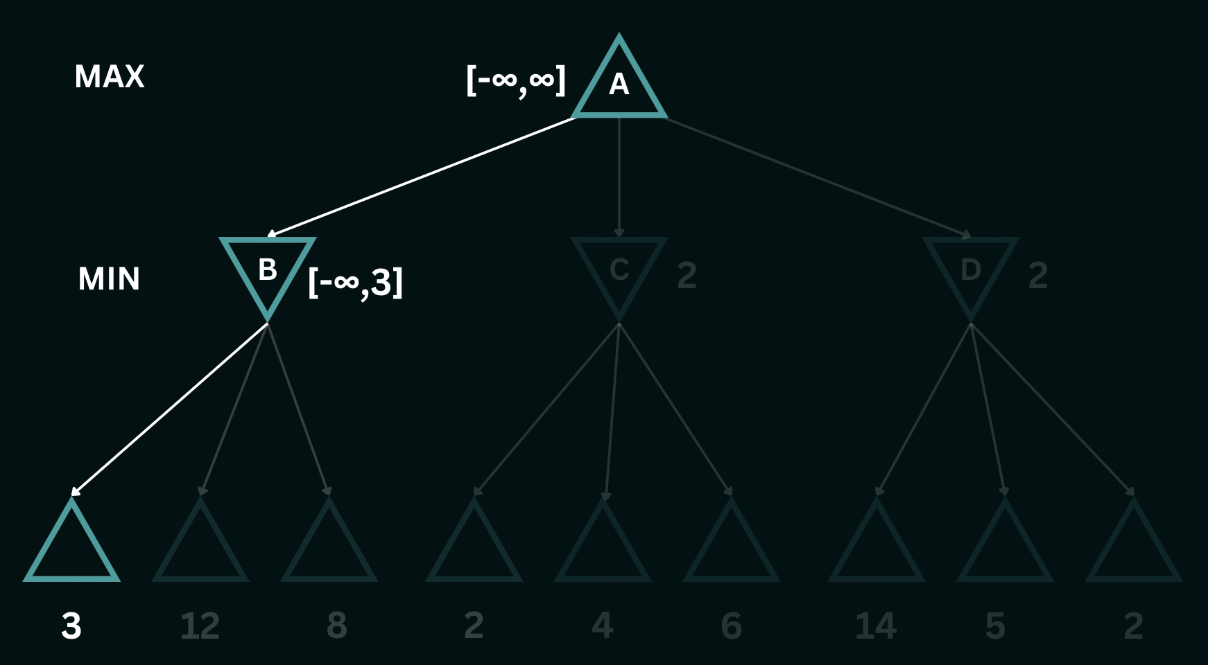
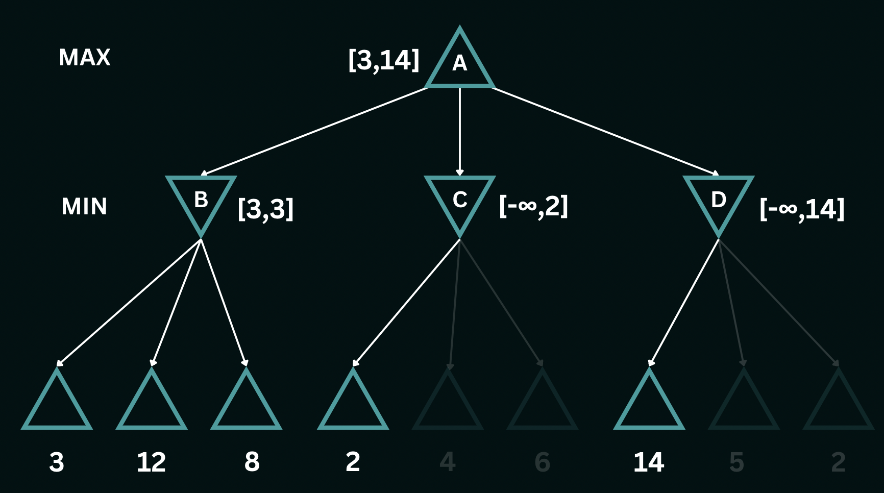
		return beta

To better understand the alpha-beta pruning algorithm, consider the same game tree as before. We initiate a recursive depth-first descent, and first encounter the leftmost leaf node of the tree, with a utility value of $3$. This sets the initial bounds for the utilities of node $B$ to $[-\infty, 3]$, indicating that the utility at node $B$ can be at most $3$. As we explore the other two branches leading to values $8$ and $12$, the $\texttt{MIN}$ player recognizes that both these moves would lead to higher scores than its initial bounds and therefore avoids playing them. Having examined all branches of node $B$, we can confidently assert that the utility is precisely $3$, i.e. the utility is bounded as $[3, 3]$. Additionally, we can infer that the utility at node $A$ is now at least $3$, i.e. the utility is bounded by $[3, \infty]$.

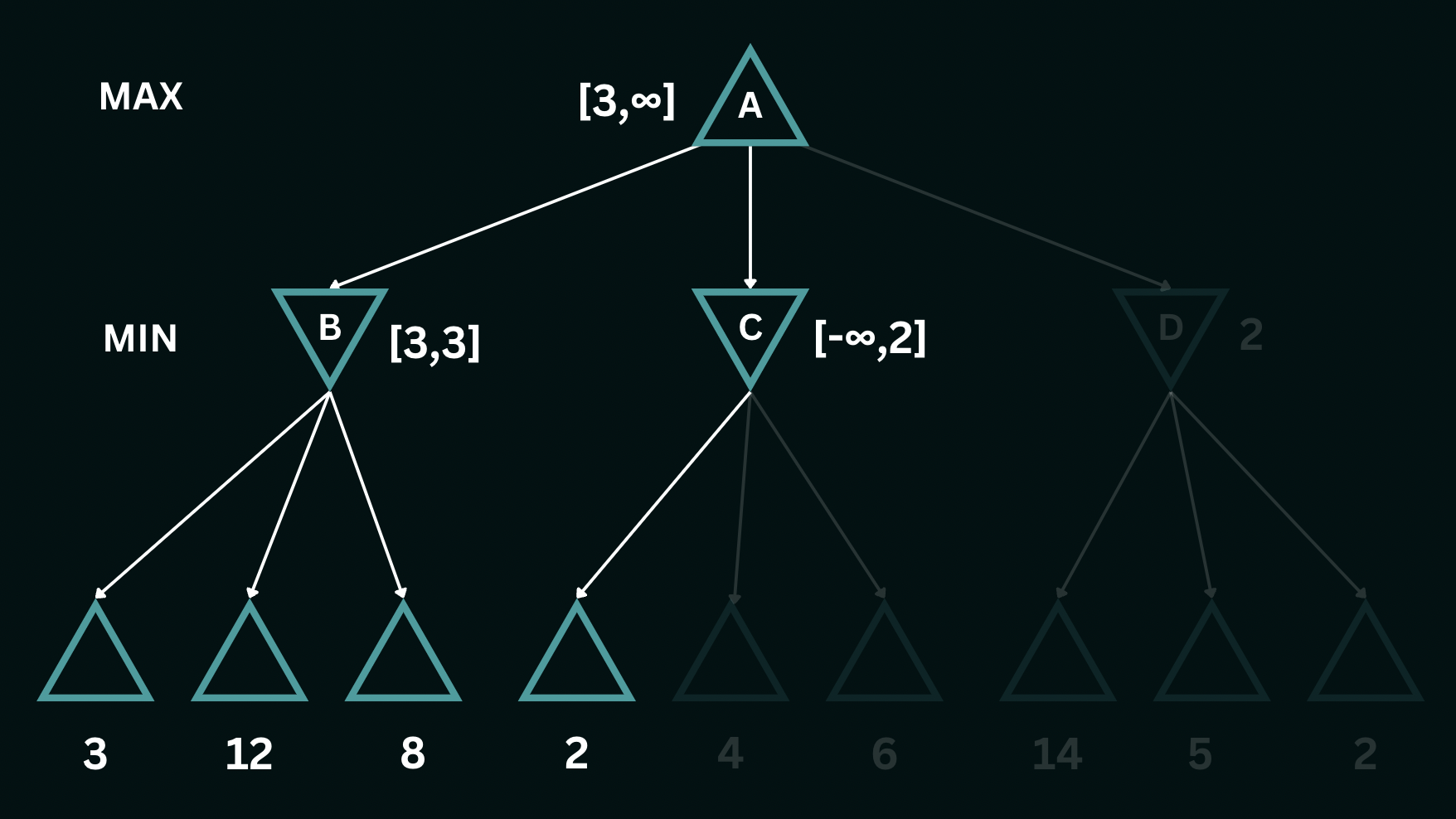
Moving on to node $C$, upon exploring its first branch, we establish the bounds for the utilities here as $[-\infty, 2]$, implying that the values can be at most $2$. However, given that the bounds at node $A$ only allow it to choose a value greater than or equal to $3$, node $C$ is never selected by the $\texttt{MAX}$ player in the decision-making process, thereby pruning the remaining two leaf nodes below $C$. Continuing our exploration, we descend into the leaves at node $D$, where the leftmost value encountered is $14$. This provides an upper bound of $14$ for the node $D$, in turn, setting the maximum value for the $\texttt{MAX}$ player at $14$. The utilities at the top are now bounded by $[3, 14]$. Recognizing that $14$ surpasses the alternative value of $3$, we proceed to explore the remaining nodes within $D$.

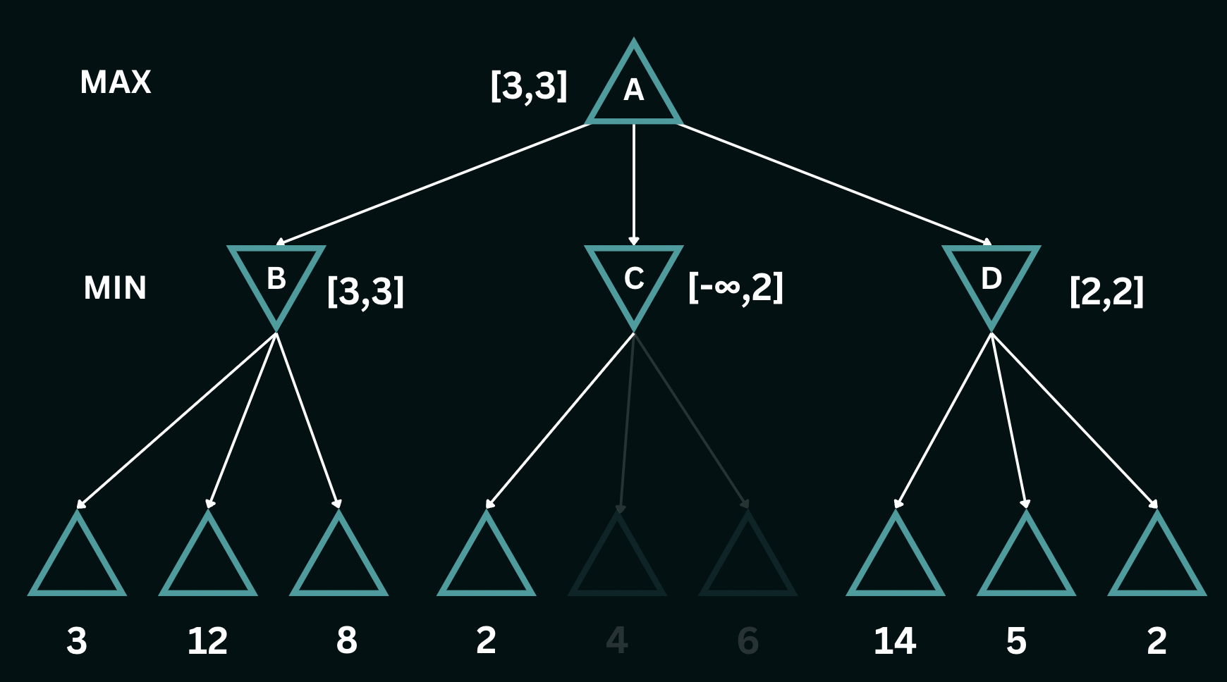
Upon exploring the remaining leaves at $D$, we eventually encounter a utility of $2$ and set the bounds at $D$ as $[2,2]$. The bounds on $A$ subsequently get restricted to a utility of exactly $3$. Note that the path that $\texttt{MAX}$ chooses remains the same as in $\texttt{MINIMAX}$ but alpha-beta pruning helps avoid expanding the two irrelevant nodes from $C$.

Constraint Satisfaction Problems

Constraint Satisfaction Problems (CSPs) are a subset of search problems that involve finding values or assignments for a given set of variables such that they satisfy a set of constraints or conditions. To define a CSP, we need to specify the following components:

1. Variables: A set of variables, which represent the unknowns. These are the values we try to optimize.
2. Domains: A set of values that each variable can take on. Each variable has its own associated domain.
3. Constraints: Constraints are restrictions or conditions limiting the possible assignments of values to variables.

An assignment is the mapping of specific values to variables within a problem. A consistent or legal assignment is one in which the chosen values for the variables adhere to all specified constraints, ensuring that no constraint is violated. Assignments do not always have to include all variables (especially when a problem has conflicting constraints that can not be true at the same time). An assignment can be partial (i.e., it covers a subset of variables) or it can be complete (covers all variables).

To find a solution to a constraint satisfaction problem is to find a complete and consistent assignment. When this is not possible, we seek a partial solution, which is a partial assignment that remains consistent with respect to constraints concerning the assigned variables. To reinforce our understanding, let us consider a real-world example. Consider the game of Sudoku, which we will now represent as a CSP. The rules of the game dictate that each cell in the 9x9 grid is populated in such a way that the value in a given cell is unique within the row and column, as well as the 3x3 subgrid the cell is in. The variables in this scenario are the entries in each cell. The domain of each cell is the set of digits from 1 to 9. The following is an example of how one may represent Sudoku as a CSP:

• Variables: $X_{ij}$, where $i$ is the row and $j$ is the column.
• Domains: $X_{ij}\in\{1, 2, \dots, 9\}$
• Constraints:
• $X_{ij}\ne X_{ik}\; \forall\ j\ne k$ [Row Constraint]
• $X_{ij}\ne X_{kj}\; \forall\ i\ne k$ [Column Constraint]
• $X_{ij}\ne X_{kl}\; \forall\ (i, j)\ne (k, l), \{X_{ij}, X_{kl}\} \in S_n$ [Subgrid Constraint, $S_n$ represents the $n^{th}$ subgrid]

As a second example, we consider map-coloring or graph-coloring problems. Here, the variables are the regions on a map or the nodes in a graph, and the domain for each variable is a set of colors. The constraints are that no two adjacent regions/nodes can have the same color. The goal is to find a coloring of the map such that no two adjacent regions have the same color. This CSP type finds applications in cartography, but the general structure extends beyond maps, such as frequency assignments in wireless communications! The following is an example of how one may represent map-coloring as a CSP:

• Variables: $X_i$, where $i$ is the region/node.
• Domains: $X_i\in\{R, G, B, Y\}$
• Constraints:
• $X_i\ne X_j\; \forall\ (i, j)\in E$, where $E$ is the set of edges in the graph, or adjacent regions on a map.

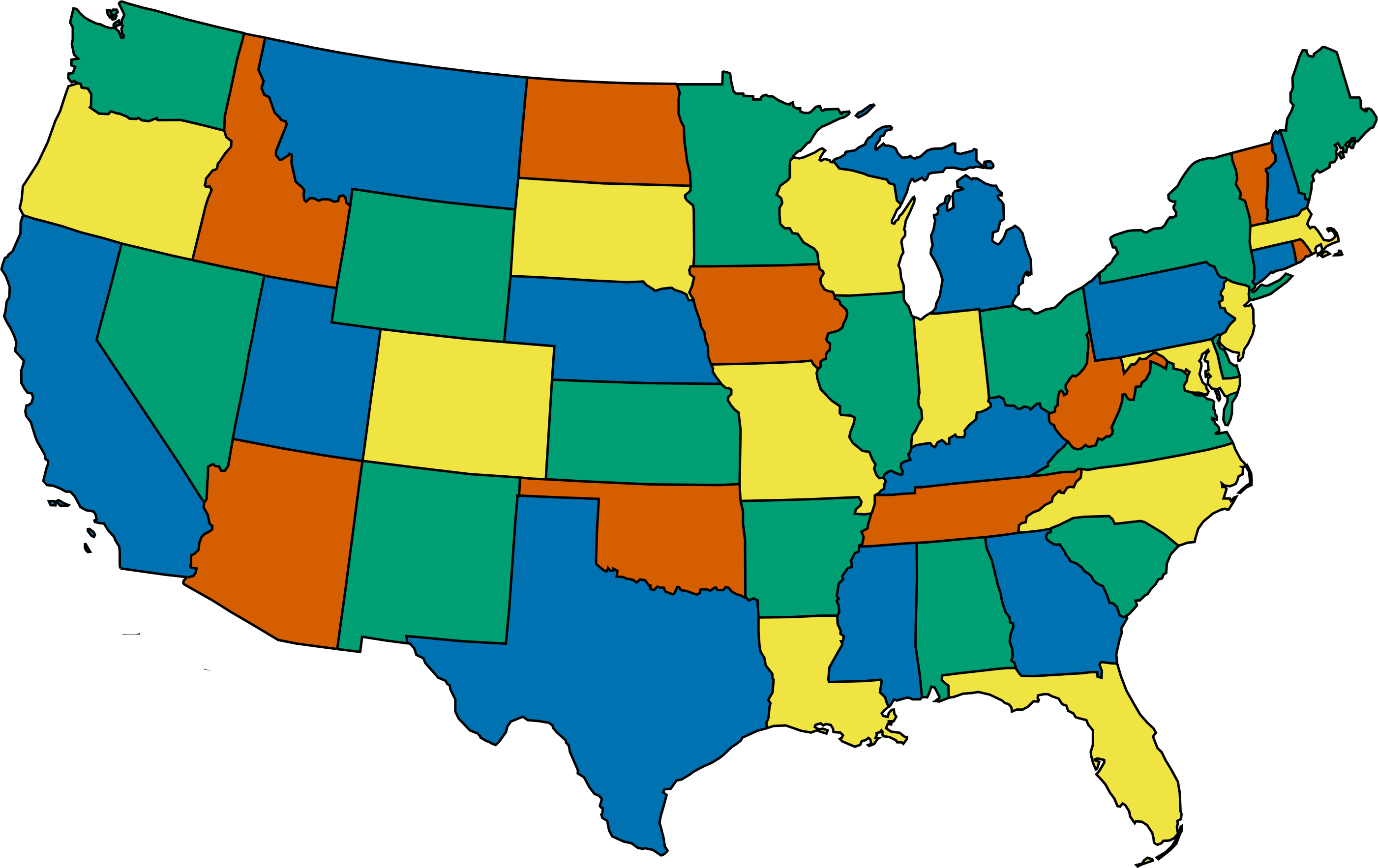
An example of a solved map-coloring problem is the following map of the contiguous United States using four colors. Note how no states that share a border are colored the same.

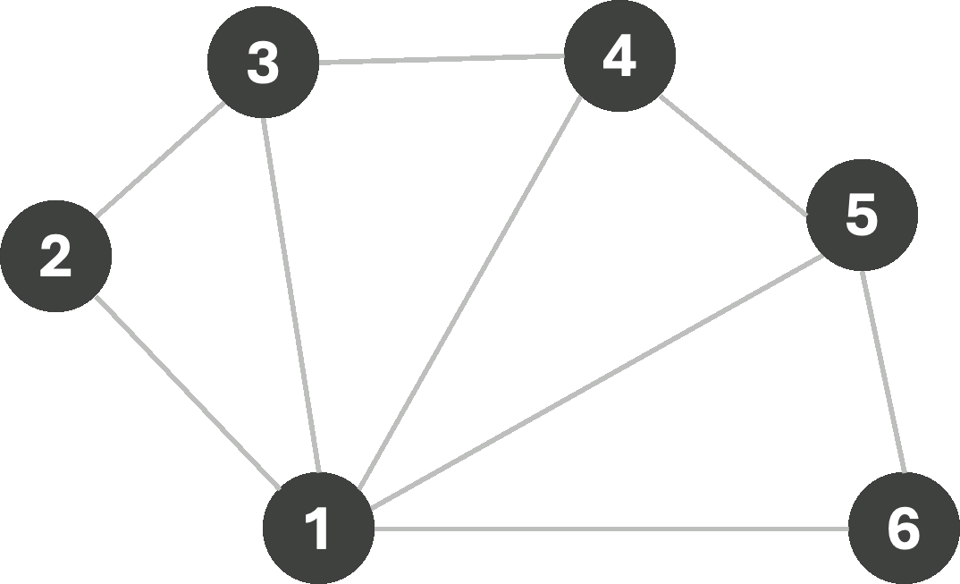
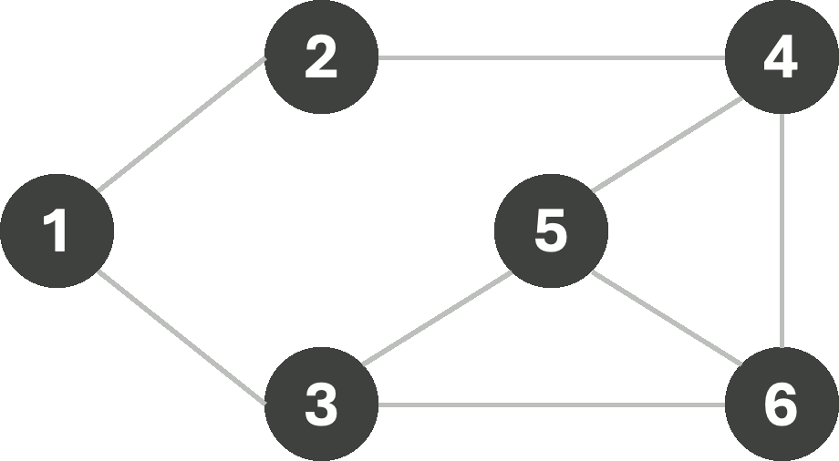
To solve a CSP (including, but not limited to graph-coloring) one may employ search algorithms. Consider the following graph:

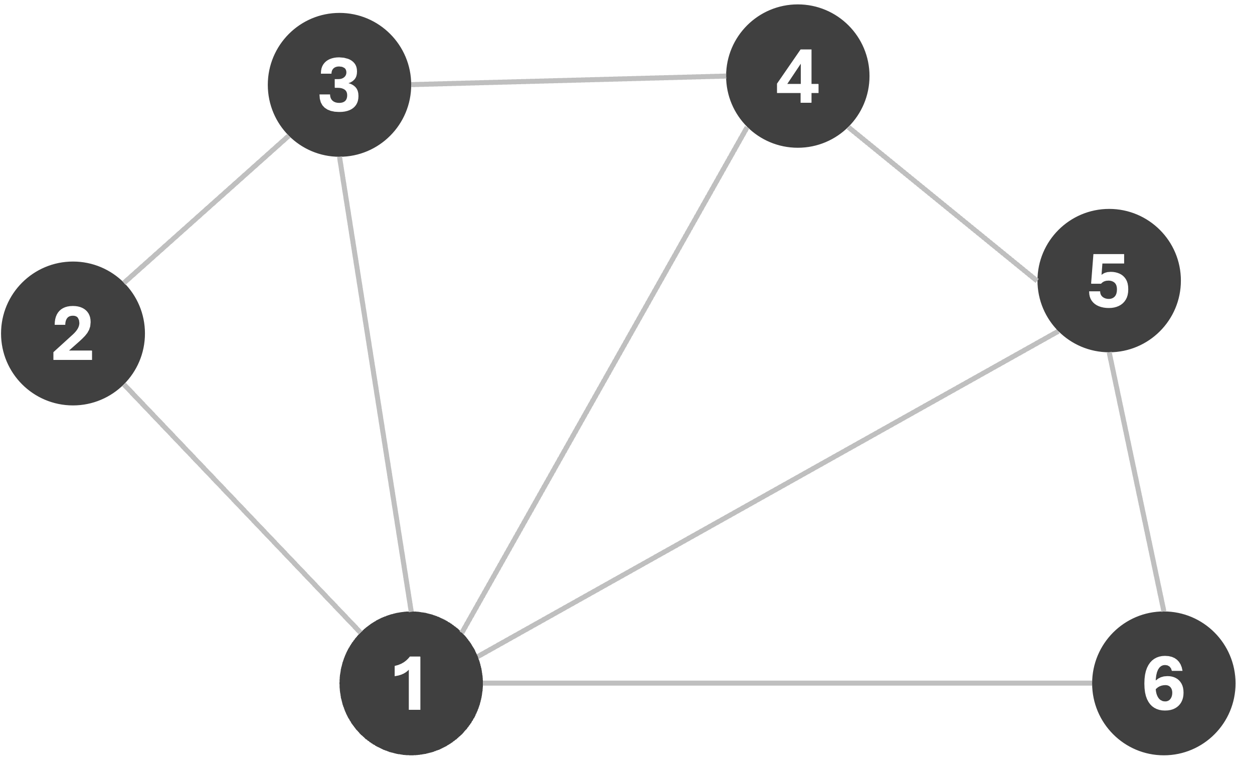
Let us first begin with a simple Breadth-First search, with the following logic: we will start assigning colors sequentially from the set [R,G,B,Y]* as we explore nodes, only making sure that the assigned color does not violate any edge-constraints. If a constraint is violated, we simply try the next color instead. If we begin our search from node 1, we get the following sequence of assignments:

*Color variants chosen to maximize contrast under common forms of color-blindness as best as possible. In case of accessibility issues, please let me know using this anonymous form, and I will make sure to update color-choices wherever necessary.

We managed to find a valid 4-coloring of this graph. However, often, the goal is not only to find any constraint-satisfying coloring, but rather the coloring that uses the fewest colors possible. Now consider the same graph, but let us instead change how we assign colors. This time, we always assign the first available color in the list with the goal of re-using colors wherever possible, aiming to minimize the number of colors used. In this scenario, we get the following coloring sequence:

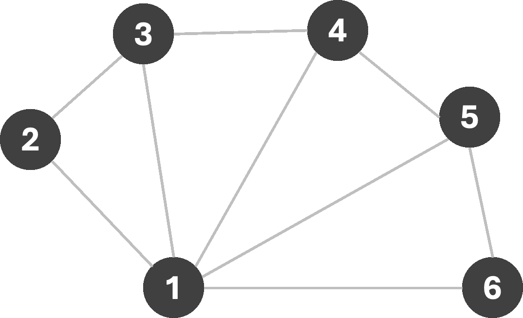
As we can see, we managed to find a 3-coloring of the graph, which is the smallest number of colors possible for this graph. This is an example of a greedy algorithm, where we make a locally optimal choice at each step with the hope of finding a globally optimal solution. However, we can do better than rely on hope. Consider, for a moment, the following graph:

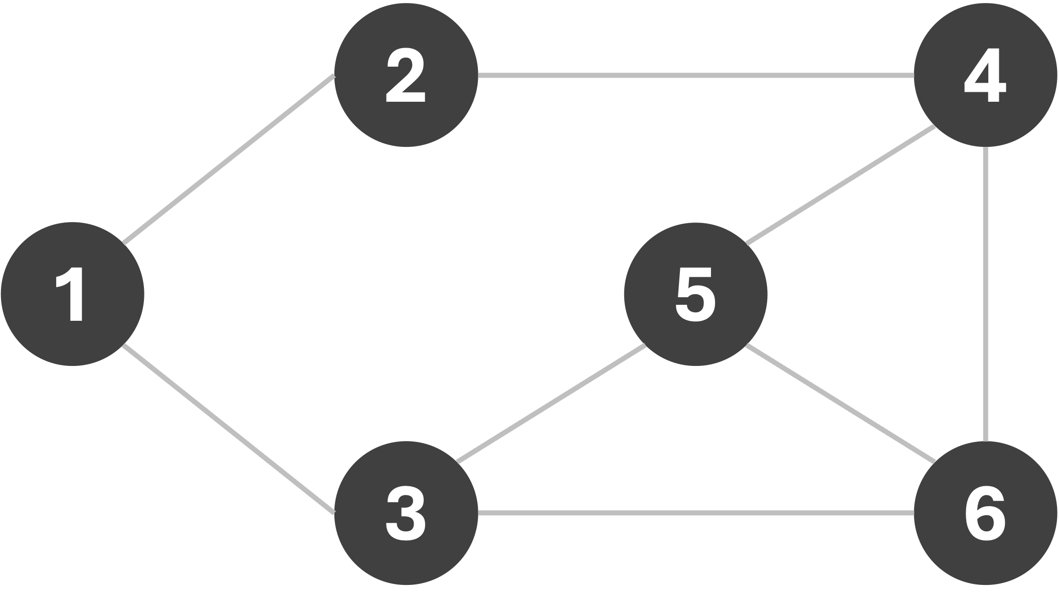
If we use the same BFS-based approach as earlier, assigning the first available color, avoiding introducing new colors unless absolutely necessary, the sequence we get depends on the node we start our search from!

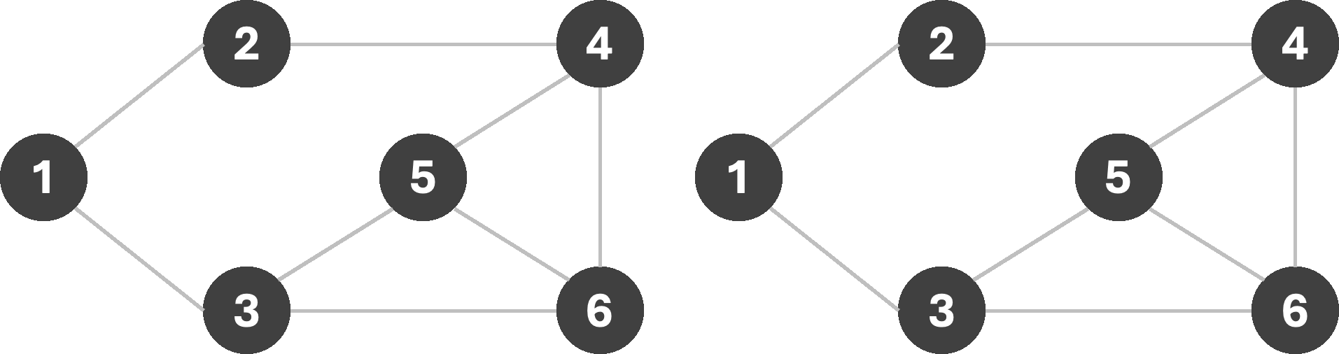
If we start our search from node 1, we are forced to use the fourth color in our set; however starting from node 5 allows us to get away with only three colors. Using the fewest available colors is often a desirable result. Note that node 5 is connected to a larger number of other nodes, and therefore helps eliminate more inconsistent assignments earlier on in the search. Properties such as node-degree (the number of neighbors), the least constraining value, etc. are often used as heuristics for constraint elimination.

For now, we make one final change to our BFS, and that is to allow backtracking. In fact, backtracking is commonly used to solve CSPs of various types, although it is perhaps easiest to demonstrate with graph-coloring problems. Consider the same search as the one on the left in the above example, starting from node 1. If we remove the fourth color (Y) as a choice from our color-set, then our search algorithm will be forced to undo a previous assignment, and try the next available color in its stead. Let us finally see how BFS with backtracking would give us the optimal coloring (3-coloring) on this graph.

Expectiminimax

While the $\texttt{MINIMAX}$ algorithm is powerful, it is limited to deterministic games. In many real-world scenarios, the environment is stochastic, and the outcome of an action is not always certain (such as a coin toss or a dice roll). In such cases, the $\texttt{EXPECTIMINIMAX}$ algorithm is used to reason about the game tree, accounting for the uncertainty in the environment. The $\texttt{EXPECTIMINIMAX}$ algorithm is a generalization of the $\texttt{MINIMAX}$ algorithm, and is used to model games using chance nodes, where the outcome of an action leads to one of several states with some associated probabilities. As the name suggests, the $\texttt{EXPECTIMINIMAX}$ algorithm is used to find the strategy that will be optimal on average. The algorithm is recursive, and can be summarized as follows:

function EXPECTIMINIMAX(node, depth, player):

	if depth = 0 or node is terminal:
		return UTILITY(node)

	if player == MAX:
		U = []
		for every child of node:
			U.append(EXPECTIMINIMAX(child, depth - 1, MIN))
		return max(U)

	else if player == MIN:
		U = []
		for every child of node:
			U.append(EXPECTIMINIMAX(child, depth - 1, MAX))
		return min(U)

	else: // chance node
		U = []
		for every child of node:
			U.append(PROBABILITY(child)*EXPECTIMINIMAX(child, depth - 1, MAX))
		return sum(U)

Consider the following game: there are two biased coins, A and B, and two players, $\texttt{MAX}$ and $\texttt{MIN}$. $\texttt{MAX}$ plays first, by choosing one of the two coins, tossing it and recording the result. The coin is then replaced, after which $\texttt{MIN}$ chooses one of the two coins, tosses it and records the result. If the two results are different, then $\texttt{MAX}$ wins, and if the results are the same, then $\texttt{MIN}$ wins. If coin A turns up heads 75% of the time, and coin B turns up heads 40% of the time, which coin should $\texttt{MAX}$ choose to flip first?

To solve this, we first draw a game-tree, this time including chance nodes, where each branch represents one possible outcome, with an associated probability. In order to have a notion of scoring, we need to assign a numerical value to each leaf node. Note that our game is zero-sum, i.e., if $\texttt{MAX}$ wins, then $\texttt{MIN}$ loses and vice-versa. We can therefore assume that leaf nodes at the end of a path traversed using different outcomes on the two coins lead to a positive score ($\texttt{MAX}$ wins), and a negative score of equal magnitude for paths with the same outcome. For simplicity, assume these scores are $10$ and $-10$ respectively. We thus obtain the following game tree.

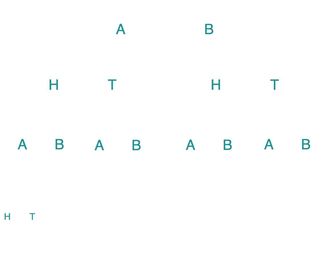
Each circle represents a chance node, denoting the probability of heads and tails at the two branches respectively. In order to find the best move for $\texttt{MAX}$, we start at the bottom. Consider the first two leaf nodes. Since the coin tossed before the parent chance node is coin A, we know that $P(H)=0.75$ and $P(T)=0.25$. The expected value of tossing the coin A, therefore, is $(-10) P(H) + (10)P(T) = (-10)(0.75) + (10)(0.25) = -5$.

Similarly, the expected value of tossing coin B is $(-10)(0.4) + (10)(0.6) = 2$. Now moving upward, the player who has to choose between these two outcomes is $\texttt{MIN}$. If we assume both players play optimally, then we can say confidently that $\texttt{MIN}$ will choose coin A as long as $\texttt{MAX}$ tossed a H on the first coin. If $\texttt{MAX}$ tossed a T instead, then the utilities at the bottom change signs, and therefore $\texttt{MIN}$ will choose coin B instead. The values under $\texttt{MIN}$ in the right half of the game-tree are the same as the left half, since $\texttt{MIN}$'s choice only depends on the outcome of $\texttt{MAX}$'s choice, and not on which particular coin led to that specific outcome.

We can then similarly compute the expected utilities of tossing coin A and B respectively for $\texttt{MAX}$, assuming that $\texttt{MIN}$ will always steer the game towards the branch where the score is minimized. The expected utility on the left branch is computed as $\mathbb{E}_{max}(A) = P(H|A)\ \mathbb{E}_{min}(H) + P(T|A)\ \mathbb{E}_{min}(T)$. Similarly for the right branch, $\mathbb{E}_{max}(B) = P(H|B)\ \mathbb{E}_{min}(H) + P(T|B)\ \mathbb{E}_{min}(T)$. The expected values propagated up to the $\texttt{MAX}$ level are shown below.

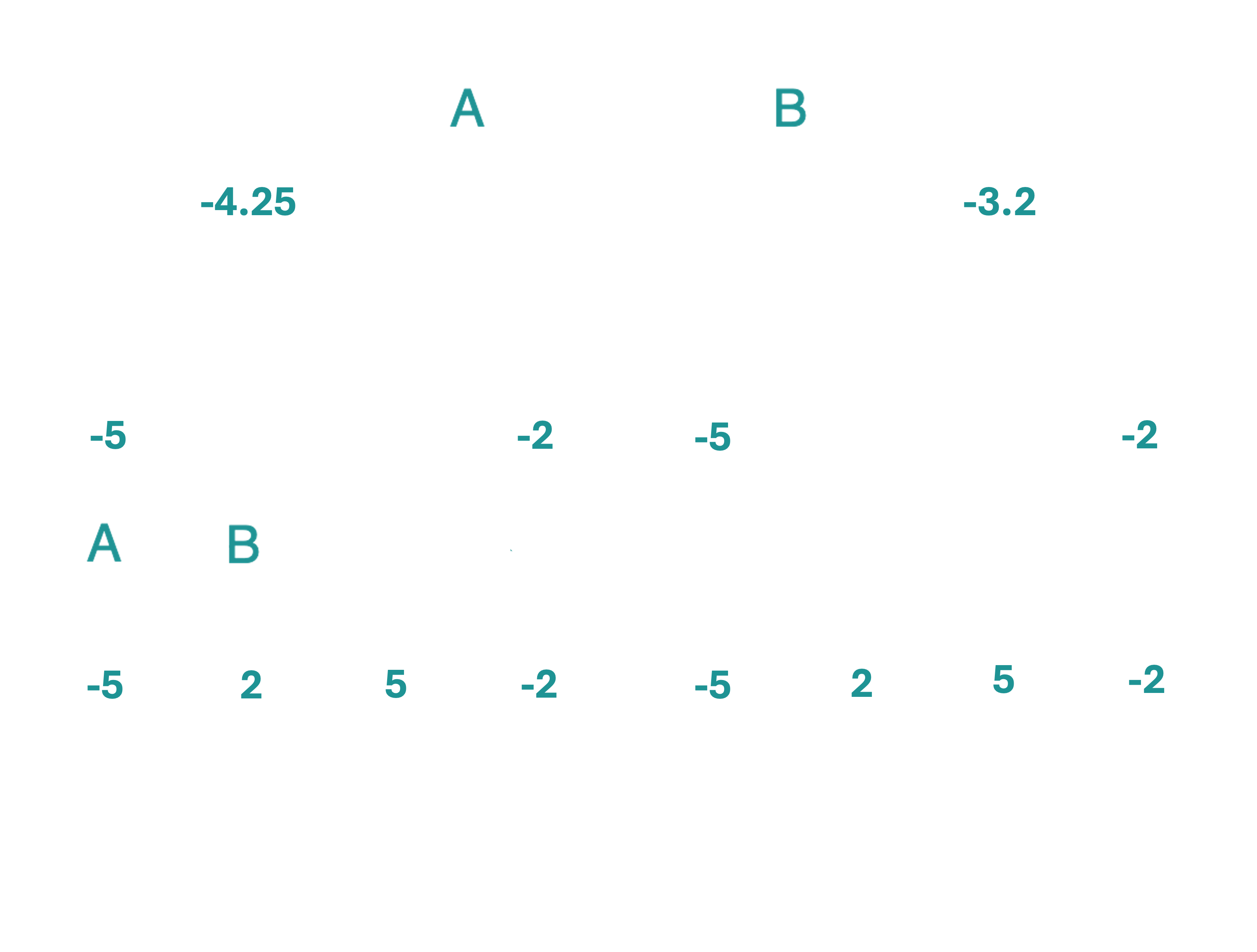
From the game tree, two things are clear: a) Playing coin B will be optimal for $\texttt{MAX}$ on average, and b) this particular game is biased against $\texttt{MAX}$. Can the probabilities of the two coins ever be adjusted such that the game is biased against the second player? Food for thought!