Probabilistic Reasoning
So far we have discussed search algorithms and developed a probabilistic reasoning model for cases where our world is static. Now, consider, for instance, the example of monitoring patients for food intake and insulin based on blood sugar levels. In this case, we encounter a shift from static to dynamic environments. Unlike static scenarios where the state sequence remains unchanged, dynamic environments introduce variability over multiple time intervals, requiring a different modeling approach. To tackle this, we adopt discrete-time models, dividing time into slices to capture snapshots of the state space at specific intervals. This enables us to observe states and make predictions based on these discrete time increments. Integral to this approach is the construction of transitional models, representing the probability distribution of the next state based on the current states.
Markov Models
Let us begin by imagining the problem of predicting whether it will rain today based on past weather data. We establish a transitional model denoted as $P(X_t | X_{0:t-1})$, where $X$ represents the weather state. However, considering an unbounded history poses an immediate challenge, as the value of $t$ increases. As time progresses, the history becomes increasingly extensive, making computations impractical. To address this, we leverage the Markov assumption, which states that the probability of the current state depends only on a finite series of previous states. As a special case, this assumption gives rise to the Markov chain representation, asserting that future state predictions are conditionally independent of the past given the present state- $P(X_t | X_{t-1})$.
However, even within the Markov assumption, there exists the issue of $t$ taking infinite values. To mitigate this, we adopt a time-homogeneous approach, assuming that the process of state transitions remains constant over time. In essence, this implies that the conditional probability of transitioning from one state to another remains consistent across all time steps. In the context of weather prediction, for example, this means that the likelihood of rain today, given the weather yesterday $P(R_t | W_{t-1})$ remains constant over all values of $t$, requiring the specification of only one transition table. By embracing these assumptions, we can effectively navigate dynamic problem spaces, enabling better decision-making. Here is an example of a Markov chain, where $X_t$ is the state variable at a time-step $t.$
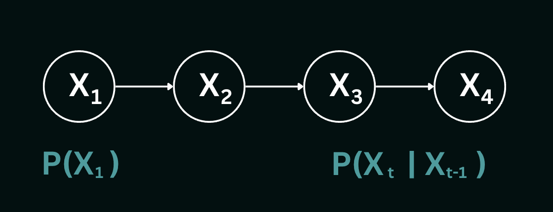
The joint distribution of the time slices $X_1$ to $X_4$ is represented by:
$$P(X_1,X_2,X_3,X_4)= P(X_1)P(X_2|X_1)P(X_3|X_2)P(X_4|X_3)$$
This equation can be further generalized into:
$$P(X_1,X_2,X_3,X_4......X_T)$$
$$ = P(X_1)P(X_2|X_1)P(X_3|X_2)P(X_4|X_3).......P(X_T |X_{T-1})$$
$$ =P(X_1) \prod_{t=2}^T P(X_t |X_{t-1})$$
Let us revisit the example of the weather model, and understand the intuition behind these probability distributions as computed using a first-order Markov assumption. The following image depicts the probability transition table over the pairs of weather conditions:
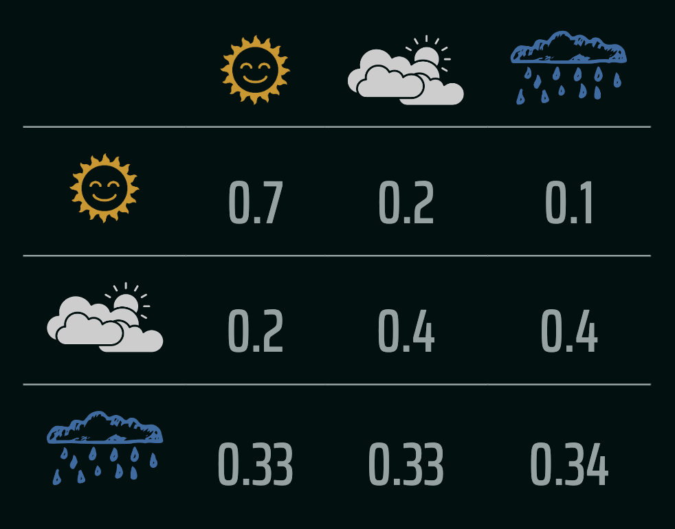
The transition probability matrix, $$P= \begin{bmatrix} 0.7 & 0.2 & 0.1\\ 0.2 & 0.4 & 0.4\\ 0.33 & 0.33 & 0.34\\ \end{bmatrix}$$ represents the probabilities of transitioning between the weather states. For example, $P[1][2] = 0.4$ means there's a $40\%$ chance of transitioning from cloudy to rainy in one time-step. The rows in general represent the states at time step $t$ and the columns are state probabilities of what happens at time step $t+1$. Therefore to represent a Markov process in terms of the transition matrix, we would have to compute $p_{ij} = P(X_{t+1} = j | X_{t = i})$. Since given the weather today, one of the three weather conditions must occur tomorrow (collectively exhaustive events), the rows must add up to one.
Given an initial probability distribution over states ($1$ through $n$) $\pi=[P(X_0 = 1), P(X_0 = 2), \dots, P(X_0 = n)]$, we compute the probability distribution of the states at the next time step by generalizing the probability distribution at time step $t$ with the equation: $$\pi_t=\pi_{t-1}P$$ When $t\rightarrow \infty$, we notice that our probabilities converge to what is known as the stationary distribution, following which the distribution does not change - it satisfies the equation $\pi=\pi P$. Let us explain these properties with the weather example. Assume that the initial probability distribution we have is, $\pi_0=[0.4,0.4,0.2]$ - indicating that there is a $40\%$ chance of a sunny day, $40\%$ chance of a cloudy day and $20\%$ chance of rain. Given this information, the distribution at time-step $1$ would look like: $$ \begin{align*} \pi_1&= \pi_0P\\ &=\begin{bmatrix}0.4 & 0.4 & 0.2 \end{bmatrix} \times \begin{bmatrix} 0.7 & 0.2 & 0.1\\ 0.2 & 0.4 & 0.4\\ 0.33 & 0.33 & 0.34\\ \end{bmatrix} \\&=\begin{bmatrix}0.426 &0.306 & 0.268\end{bmatrix} \end{align*} $$ Upon multiple sequential iterations of the above, we eventually reach some distribution $\pi$ which satisfies the equation $\pi=\pi P$. For this case, the stationary distribution is as follows: $$ \pi=\begin{bmatrix}0.46397188 &0.28998243 &0.24604569\end{bmatrix} $$ In the context of Markov chains, eigenvectors and eigenvalues provide insights of the long-term behavior of the chain. The eigenvector $v$ represents the stationary distribution much like the one we computed above, while the matrix $A$ is the transition probability matrix. If $Av=\lambda v$ is satisfied, we say that $v$ remains unchanged in direction when multiplied by the transition matrix $A$. Instead, they only get scaled by a factor of $\lambda=1$.
To reason about longer chains of events into the future (e.g., if the weather is sunny today, what will the weather be like in 10 days?), we can leverage the concept of the Chapman-Kolmogorov equation. This equation allows us to compute the probability of transitioning from state $i$ to state $j$ in $n$ time-steps. The equation is given by: $P_{ij}(n)=P^n_{ij}$. For a detailed explanation, please refer to these notes by Dr. Fewster from the University of Auckland. For Markov models where a path exists between any two states, $\lim_{n \rightarrow \infty} P^n$ converges to the stationary distribution $\pi$, with the value in the $i^{th}$ column of $P^n$ being the same as the $i^{th}$ entry in $\pi$. This essentially means that the starting state is immaterial in the long run. However, when the Markov model has terminal or absorbing states, from which a random walk cannot depart, this is no longer the case. Consider, for example, the problem of the gambler's ruin. In this scenario, a gambler starts with $k$ units of money and plays a game where he wins or loses a unit of money each round with equal probability. The game ends when the gambler has no money left or when he has $t$ units of money. Assuming $i \in \{25,50\}$ and $t=75$, we get the following Markov model:
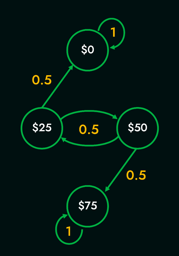
$$P= \begin{bmatrix}
1 & 0 & 0 & 0\\
0.5 & 0 & 0.5 & 0\\
0 & 0.5 & 0 & 0.5\\
0 & 0 & 0 & 1
\end{bmatrix}$$ is the initial transition matrix. To compute the probability of exiting the game with a $\$0$ given that the player starts with $\$25$ after two time-steps is essentially given by $P^2(\$0 | \$25)$. The transition matrix after two time-steps would look as follows:
$$
P^2=\begin{bmatrix}
1 & 0& 0& 0& \\
0.5 & 0.25& 0& 0.25\\
0.25 &0& 0.25 &0.5 \\
0& 0& 0& 1 \end{bmatrix}
$$
The probability $P^2(\$0 | \$25)=0.5$. Additionally, as $t\rightarrow\infty$, we would get the following computed matrix consisting of the stationary distribution:
$$
P^\infty=\begin{bmatrix}
1 & 0& 0& 0& \\
\frac{2}{3}& 0& 0& \frac{1}{3}\\
\frac{1}{3} &0& 0 &\frac{2}{3} \\
0& 0& 0& 1 \end{bmatrix}
$$
This game illustrates that to have a higher chance at winning, one is incentivized to start with a larger sum of money. This is because the probability of winning the game converges to the stationary distribution, which is higher for a larger initial sum of money. With a larger number of states between $\$0$ and the target amount, the probability of winning the game shifts significantly towards a larger initial pot. Remember that so far we've only considered an unbiased game. If the game is biased, the transition matrix would change accordingly.
Hidden Markov Models
In real-world scenarios like voice recognition, genetic sequence alignment, or predicting stock prices, accurately estimating the probability distribution over the next possible states is crucial. However, this information is often not directly accessible. Instead, our agents gather observations over time, which they use to update their beliefs about the environment. To accommodate this, we need to update our Markov models to incorporate the observations received by the agent at each time step. In practical settings, our models must adapt to the dynamic nature of the environment by integrating observed data into the modeling process. For instance, in voice recognition, the hidden states may represent phonemes or words, while the observations consist of acoustic features. As the agent listens to speech, it collects these observations over time and updates its belief about which sequence of hidden states is most likely to have generated the observed data.
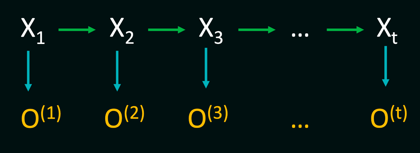
A Hidden Markov Model consists of three fundamental components: the initial distribution $P(X_1)$, transition probabilities denoted by $P(X_t∣X_{t−1})$, and observation/emission probabilities $P(O_t∣X_t)$. Additionally, HMMs operate under two critical Markov assumptions:
- Temporal Dependency: The future states of the system depend solely on the present state, encapsulated by the transition probabilities $P(X_t∣X_{t−1})$. This implies that the sequence of states forms a Markov chain, where the probability distribution of the next state depends only on the current state.
- Observational Independence: Given the current state, the observation at a particular time step is independent of all other observations and states in the sequence, apart from the current state. This independence is described by the emission probabilities $P(O_t∣X_t)$.
Now, let us consider the HMM example from class, where the true states denote whether the professor's train is very late, late or on time, and the observations are the professor's mood - either happy or sad. The following diagram shows the various transitions between states, and emissions from states to observations.
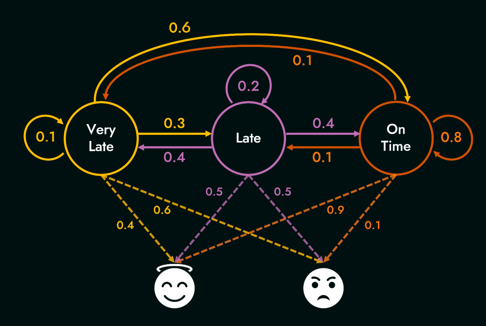
Here are the state transition matrix $T$ and the emission/observation matrix $O$ respectively:
| Very Late | Late | On Time | |
| Very Late | 0.1 | 0.3 | 0.6 |
| Late | 0.4 | 0.2 | 0.4 |
| On Time | 0.1 | 0.1 | 0.8 |
| Happy | sad | |
| Very Late | 0.4 | 0.6 |
| Late | 0.5 | 0.5 |
| On Time | 0.9 | 0.1 |
Given a set of these probabilities, we can deduce three types of reasoning using an HMM [Rabiner, L. R’s HMM tutorial, 1989].
- Probability of observing a sequence: Given an HMM with parameters $\lambda = (T, O, \pi)$ and an observation sequence $o$, determine the likelihood of $P(o|\lambda)$.
- Most likely sequence, given observations: Given an HMM with parameters $\lambda = (T, O, \pi)$ and an observation sequence $o$, determine the most likely hidden sequence, $q$. In other words, find $$\arg\max_{q} P(o|q)$$
- Finding model parameters that best explain observations: Given an observation sequence $o$ and the set of states in the HMM, learn the HMM parameters $T$ and $O$.
Type 1
Let us start with the first type of reasoning. Given both a sequence of observations, and the corresponding hidden states, calculating the joint probability is fairly straightforward. For a particular hidden state sequence $q = q_0,q_1,q_2,...,q_T$ and an observation sequence $o = o_1,o_2,...,o_T$ , the join probability is given by:
$$P(o,q)= \prod_{t=1}^T P(q_t | q_{t-1}) P(o_t |q_t)$$
To compute $P(q_1 | q_0)$ in the above equation (the probability of being in a specific hidden state at the first time step), we often simply resort to using the stationary distribution of the Markov chain defined over the hidden states. Thus $P(q_1 | q_0) = \pi(q_1)$. Note that this joint probability is different from the conditional probability of a sequence of observations given a sequence of hidden states. The latter is computed as $P(o|q) = \prod_{t=1}^T P(o_t |q_t)$, since the hidden-state sequence is assumed to have occurred in this setting. These are also related as $P(o,q) = P(o|q)P(q)$.
Now, consider the case where we compute the probability of an observation sequence $o$, not knowing the hidden sequence $q$. In this scenario, we need to account for all possible hidden-state sequences, and sum over their joint probabilities with the observation sequence. Intuitively, we can think of this as follows - consider a set of 3 observations $o=o_1, o_2, o_3$. Any possible hidden-state sequence $q = q_1, q_2, q_3$ could have given rise to these observations; however, only one of these hidden-state sequences will occur in a single random sample of length 3 from the HMM. We therefore sum over the joint probabilities of all such hidden-state sequences along with the observation sequence to get the total probability of the observation sequence. This is given by: $$P(o) = \sum_{q} P(o|q) P(q)$$ For an HMM with $N$ hidden states and an observation sequence of $T$ observations, there are $N^T$ possible hidden sequences. For real tasks, where $N$ and $T$ are both large, $N^T$ is a very large number (recall the slide with a wall of computations from class). Obviously, this is computationally very expensive; however we can exploit the fact that the probability of the observation sequence up to time $t$ can be computed using the probability of the observation sequence up to time $t-1$. This is done by summing over the probabilities of all possible hidden-state sequences at time $t-1$, and then multiplying by the transition probability to the current state, and the emission probability of the current observation. This is done recursively, and the final probability is obtained by summing over the probabilities of all possible hidden-state sequences at time $T$.
To this end, we use the Forward Algorithm which has a time complexity of $O(N^2 T)$ which uses a lookup table to store intermediate values as it builds up the probability of the observation sequence. The algorithm recursively computes total probability by implicitly folding all possible paths into a single forward trellis. The forward trellis over N time-steps is represented by the following equation: $$ \alpha_t(S_i)= \sum_{j=1}^N \alpha_{t-1}(S_j) P(S_i | S_j) P(o_t | S_i) $$ where $j$ represents the different possible hidden states at each level of the search. Note that $\alpha_t(S_i)$ is nothing but the joint probability of a sequence of observations and a hidden state at time $t$, and therefore at $t=1$, we once again rely on the stationary distribution to compute $\alpha_1(S_i)$ as: $$ \alpha_1(S_i)= \pi(S_i) P(o_1 | S_i) $$ At time $t=2$, we can compute $\alpha_2(S_i)$ as: $$ \alpha_2(S_i)= \sum_{j=1}^N \alpha_1(S_j) P(S_i | S_j) P(o_2 | S_i) $$ and so on. The final probability of the observation sequence (after $T$ time-steps) is then given by: $$ P(o) = \sum_{i=1}^N \alpha_T(S_i) $$
Let us walk through computing the likelihood of observing the sequence (happy, sad, happy) from the in-class example by breaking the tree down into smaller problems as follows:
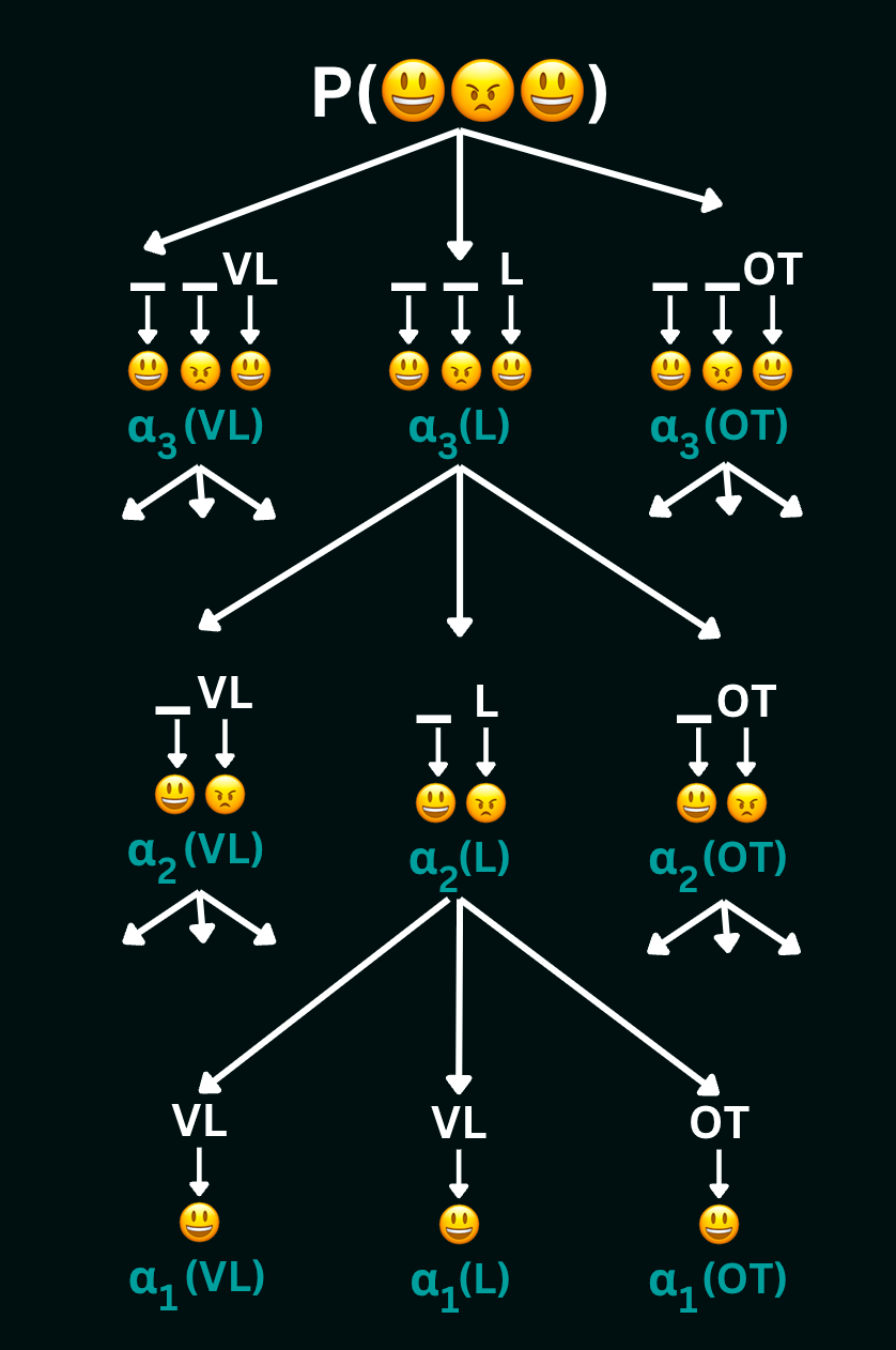
To compute $\alpha_3(VL)$ (which is the total probability of all state-sequences of length 3 ending in $VL$) using this tree, we get:
$$
\alpha_3(VL)= \alpha_2(VL)P(VL|VL)P(happy|VL)+
\alpha_2(L)P(VL|L)P(happy|VL)+
\alpha_2(OT)P(VL|OT)P(happy|VL)
$$
The values $\alpha_3(L)$ and $\alpha_3(OT)$ can be computed similarly. Then, to compute $\alpha_2(VL)$, we get:
$$
\alpha_2(VL)=\alpha_1(VL)P(VL | VL)P(sad |VL) +
\alpha_1(L)P(VL | L)P(sad | VL) +
\alpha_1(OT)P(VL | OT)P(sad |VL)
$$
The values $\alpha_2(L)$ and $\alpha_2(OT)$ can be computed similarly. Finally, to compute $\alpha_1(VL)$, we get:
$$
\alpha_1(VL)=P(VL)P(happy|VL)
$$
The values $\alpha_1(L)$ and $\alpha_1(OT)$ can be computed similarly. Thus, we calculate the forward trellis of each state sequence ending in $L$ and $OT$ at every time-step, and storing them for lookup at the next time step. Summing the values of $alpha$ at any level gives us the total probability of the observation sequence up to that time-step. Summing values at the top level gives us the total probability of the entire observation sequence. In our example, this sum is over all possible paths of length 3, and is the total probability of observing the sequence (happy, sad, happy).
Type 2
For the second type of reasoning, i.e., finding the most likely hidden-state sequence, given an observation sequence, we use a dynamic programming algorithm, called the Viterbi algorithm. This can be interpreted as a straightforward extension to the forward algorithm, where at the end of a desired observation sequence, we find the most likely hidden state by taking the max over the forward trellis, instead of summing the values. The trellis equation for the Viterbi algorithm is given by:
$$
\delta_t(S_i)= \max_{j=1}^N \bigg[\delta_{t-1}(S_j) P(S_i | S_j) P(o_t | S_i)\bigg]
$$ and the base case is once again computed using the stationary distribution as $$\delta_1(S_i)= \pi(S_i) P(o_1 | S_i)$$ The final probability of the most likely hidden state sequence $q$ after $T$ time-steps is then given by:
$$
P(q) = \max_{i=1}^N \delta_T(S_i)
$$
Let us walk through computing the most likely sequence of hidden states given the sequence (happy, sad, happy) from the in-class example by breaking the tree down into smaller problems as follows:
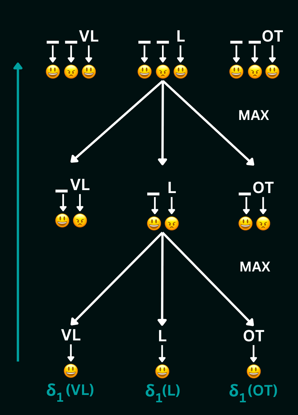
To compute $\delta_3(VL)$ (which is the probability of the most likely state-sequence of length 3 ending in $VL$) using this tree, we get:
$$
\delta_3(VL)= \max\bigg[\delta_2(VL)P(VL|VL)P(happy|VL), \delta_2(L)P(VL|L)P(happy|VL), \delta_2(OT)P(VL|OT)P(happy|VL)\bigg]
$$
The values $\delta_3(L)$ and $\delta_3(OT)$ can be computed similarly. Then, to compute $\delta_2(VL)$, we get:
$$
\delta_2(VL)=\max\bigg[\delta_1(VL)P(VL | VL)P(sad |VL), \delta_1(L)P(VL | L)P(sad | VL), \delta_1(OT)P(VL | OT)P(sad |VL)\bigg]
$$
The values $\delta_2(L)$ and $\delta_2(OT)$ can be computed similarly. Finally, to compute $\delta_1(VL)$, we get:
$$
\delta_1(VL)=P(VL)P(happy|VL)
$$
The values $\delta_1(L)$ and $\delta_1(OT)$ can be computed similarly. Thus, we calculate the Viterbi trellis of each state sequence ending in $L$ and $OT$ at every time-step, and storing them for lookup at the next time step. Taking the max of the values of $\delta$ at any level gives us the probability of the most likely hidden state sequence up to that time-step. Taking the max of the values at the top level gives us the probability of the most likely hidden state sequence of the entire observation sequence. In our example, this max is over all possible paths of length 3, and is the probability of the most likely hidden state sequence given the observation sequence (happy, sad, happy).
Markov Decision Processes
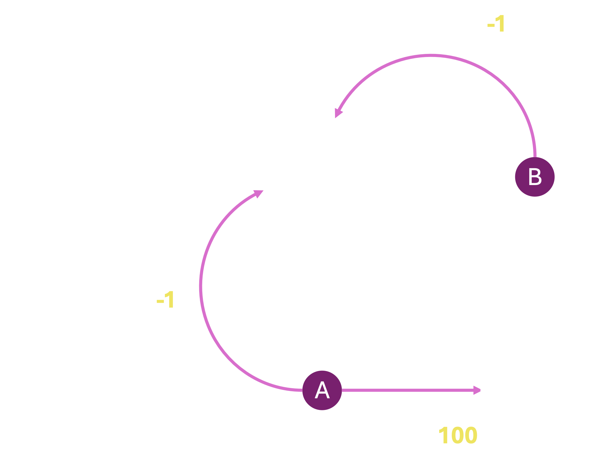
In our discussions thus far, we explored modeling dynamic environments that involve probabilistic events where outcomes are not certain but have associated transition (conditional) probabilities. We have also previously explored searches in deterministic environments, where actions lead to predictable outcomes. We now introduce stochastic environments to our search problems, where an action taken from a state is no longer guaranteed to lead to a specific successor state. Instead, we now consider the scenario where there is a probability associated with each action leading our agent from one state to another. Consider the following scenario:
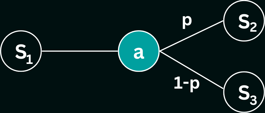
Here, from state $S1$, our agent takes action $a$, but may end up in either state $S_2$ or state $S_3$, with associated probabilities $p$ and $1-p$ respectively. In other words, $100p \%$ of the time, the agent will end up in $S_2$, and $100(1-p) \%$ of the time in $S_3$. This stochastic system can be formally represented as a Markov Decision Process (MDP), which is a mathematical model describing a problem characterized by uncertainty.
- State Space, $S$ : the set of all possible states that the system can be in. In the above example, $S = \{S_1, S_2, S_3\}$.
- Action Space, $A$ : the set of all possible actions. In the above example, $A = \{a\}$, since there is only one possible action from a state in $S$. No actions can be taken from states $S_2$ and $S_3$, and are therefore terminal or end states in the MDP.
- Transition Probabilities, $T$ : a the probabilities of transitioning from one state to another given a specific action, notated as $T(s,a,s')$, where $s$ is the source state, $a$ is the action and $s'$ is the target/successor state. In our example, $T(S_1, a, S_2) = p$, and $T(S_1, a, S_3) = 1-p$.
- Rewards, $R$ : a numerical reward associated with each transition. In general, $R(s,a,s')$ should be thought of as the reward of reaching target state $s'$ from state $s$ using action $a$.
- Discount Factor, $\gamma$ : accounts for the discounting of future rewards in decision-making. It ensures that immediate rewards are valued more than future rewards. Discounting rewards in general prevents the agent from choosing actions that may lead to infinite rewards (cyclical paths).

Evaluating Policies
In order to find the best policy for our agent, we must be able to compare two or more given policies quantitatively, to figure out which of the policies is expected to yield a higher return on average. Remember that under any one policy, every time the agent is in a state, it takes the same action; however, since the agent may end up in a different state each time (based on the values in $T$), the outcome of the policy may vary (we can stop 'playing' when the agent reaches a terminal state). This is why we need to evaluate policies in terms of their expected cumulative rewards rather than what happens in any one specific sample. A single actual path taken by the agent as a result of following a policy is called an episode. We define the utility of an episode as the discounted sum of rewards along the path. Given the episode $E = (s_0, a_0, r_0, s_1, a_1, r_1, ..., s_n, a_n, r_n, s_{END})$, the utility of the episode is given by:
$$
U(E) = \sum_{t=0}^n \gamma^t r_t
$$
where $r_t$ is the reward at time $t$, and $\gamma$ is the discount factor. The expected utility of a policy $\pi$ is then given by the expected value of the utility of the episodes generated by the policy. Given a series of episodes, the expected value is simply the average of the utilities obtained in each episode; i.e., given a set of episodes $E_1, E_2, ..., E_n$, the expected utility of the policy is given by:
$$
E[U(\pi)] = \frac{1}{n} \sum_{i=1}^n U(E_i)
$$
In practice, we are often concerned about the expected value of starting in a given state $s$ and following a policy $\pi$ from there. This is called the value of the state under the policy, and denoted $V(s)$. Here, it is useful to define a second, related quantity, called the Q-value, defined over a state-action pair. The Q-value of a state-action pair $(s,a)$ under a policy $\pi$, denoted $Q(s,a)$, is the expected utility of starting in state $s$, taking action $a$, and then following policy $\pi$ thereafter. Note that in the case where the action $a$ is also the action dictated by the policy $\pi$, then the value of the state $s$ under $\pi$ is equal to the Q-value for that state-action pair. In other words, $V_\pi(s) = Q_\pi(s,a=\pi(s))$. Finally, also note that the value of any end state is always $0$, since no action can be taken from that state.
With this in mind, we now need to find a way to calculate $Q_\pi(s,a)$. Recall that from state $s$, the agent takes action $a$, and with probability $T(s,a,s')$, it transitions to a successor state $s'$. From $s'$ the agent follows policy $\pi$, and the process continues. However, the Markov assumption allows us to simplify this process to a recurrence relation, spanning one step at a time. We can deconstruct the expected utility of starting in state $s$, taking action $a$, and then following policy $\pi$ as 1) ending up in one of several possible states $s'$, 2) receiving the immediate reward of the transition from $s$ to $s'$ using $a$, and 3) the expected utility of continuing from $s'$ and following policy $\pi$ thereafter. We need to account for all possible candidates for $s'$ for a given $(s,a)$ pair; however since only one of those candidates will be the actual successor state, we take the expected value of the utility of each candidate. This is given by the following Bellman equation: $$ Q_\pi(s,a) = \sum_{s'} T(s,a,s') \bigg[R(s,a,s') + \gamma V_\pi(s')\bigg] $$ When $a = \pi(s)$, then $Q_\pi(s,a) = V_\pi(s)$, and the value of the state under the policy $\pi$ is then given by: $$ V_\pi(s) = \sum_{s'} T(s,a,s') \bigg[R(s,a,s') + \gamma V_\pi(s')\bigg] $$ While in certain situations, the above equations may yield a closed-form solution for the value of a state under a policy, in general, we need to solve a system of linear equations to find the value of each state under the policy. This is done using a dynamic programming algorithm that iteratively computes the value of each state under the policy until the values converge. This algorithm is called the Policy Evaluation algorithm, and works as follows. We re-write the above equation to use previous estimates of $V_\pi(s)$ to compute new estimates of $V_\pi(s)$ as follows: $$ V^{(t)}_\pi(s) = \sum_{s'} T(s,a,s') \bigg[R(s,a,s') + \gamma V^{(t-1)}_\pi(s')\bigg] $$ where $V^{(t)}_\pi(s)$ is the estimate of the value of state $s$ under policy $\pi$ at iteration $t$. We start with an initial guess for the value of each state (usually set to 0), and then iteratively update the value of each state using the above equation until the values converge. Let us run through an example!
Consider the dice game example from class. The agent begins in a "start" state, and can take one of two actions: "stay" or "quit". If the agent chooses "stay", it receives a reward of \$4, and then a die is rolled. If the die roll results in a number greater than 2, the agent gets to play again, but if the die results in 1 or 2, the game ends. Equivalently, we can say that $R(\textrm{start, stay, end}) = R(\textrm{start, stay, start}) = 4$. If the agent chooses "quit" from the "start" state, it receives a reward of \$10, and the game ends; therefore $R(\textrm{start, quit, end})=10$. This game can be represented as the following MDP:
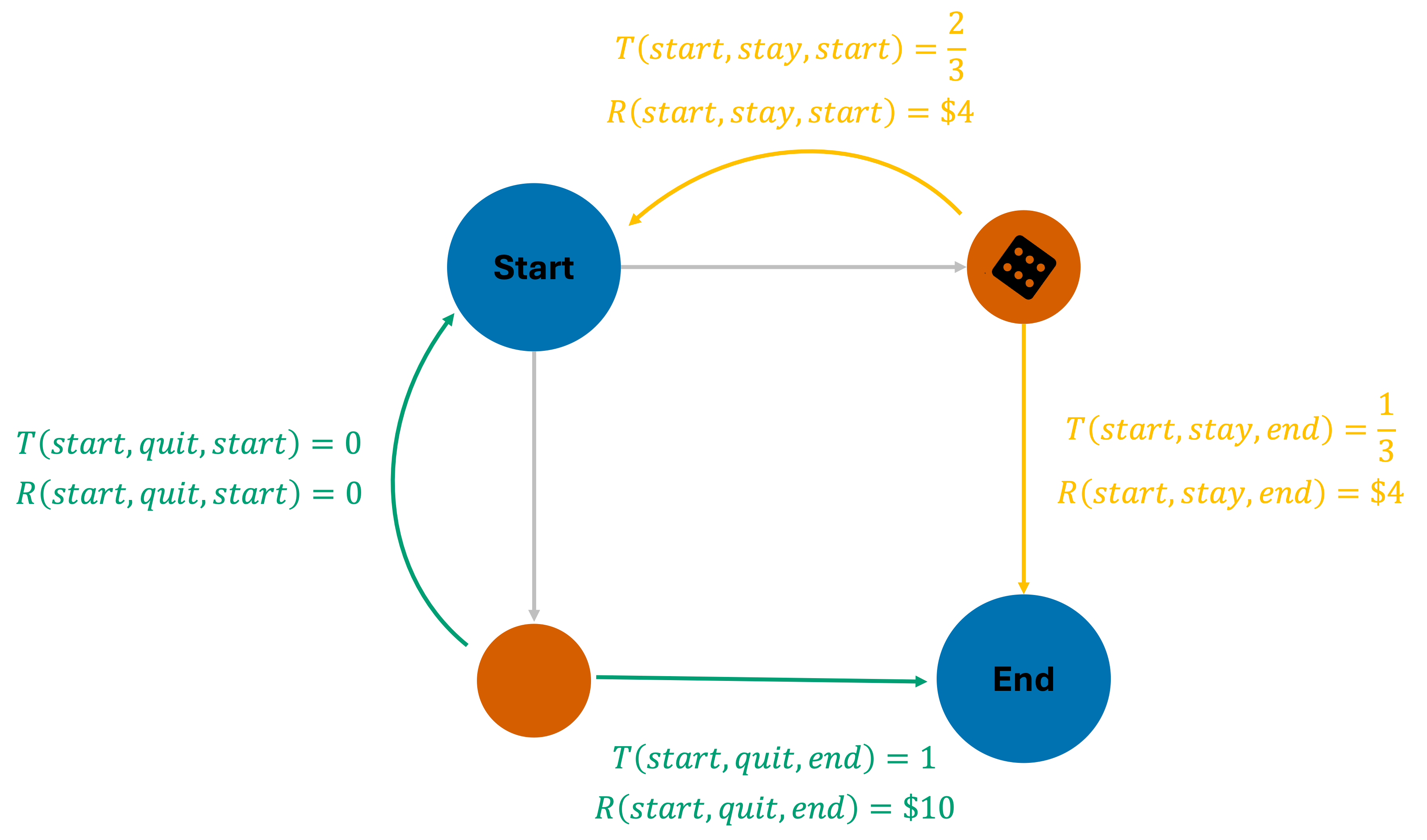
Let us now calculate the expected value of the start state, for a fixed "stay" policy, i.e., the agent always chooses to stay in the game. This is the type of policy evaluation that we are currently interested in - our goal is to find the best action for each state. Now, from the start state, given the policy $\pi = \{\textrm{start:stay, end:X}\}$, the Bellman equation can be expanded as follows: $$ V_\pi(\textrm{start}) = \sum_{s'} T(\textrm{start, stay, s'}) \bigg[R(\textrm{start, stay, s'}) + \gamma V_\pi(s')\bigg] $$ Since the "stay" action can lead us to two possible states $s'$, we can expand the above equation as follows: $$ V_\pi(\textrm{start}) = T(\textrm{start, stay, start}) \bigg[R(\textrm{start, stay, start}) + \gamma V_\pi(\textrm{start})\bigg] + T(\textrm{start, stay, end}) \bigg[R(\textrm{start, stay, end}) + \gamma V_\pi(\textrm{end})\bigg] $$ For simplicity, let us assume $\gamma=1$. We can now substitute the known values of the transition probabilities and rewards to get: $$ V_\pi(\textrm{start}) = \frac{2}{3} \bigg[4 + V_\pi(\textrm{start})\bigg] + \frac{1}{3} \bigg[4 + V_\pi(\textrm{end})\bigg] $$ Now recall that the value of an end state is always $0$, since no further actions can be taken from them. Therefore, $V_\pi(\textrm{end}) = 0$. Substituting this value into the above equation, we get: $$ V_\pi(\textrm{start}) = \frac{2}{3} \bigg[4 + V_\pi(\textrm{start})\bigg] + \frac{1}{3} \bigg[4 + 0\bigg] $$ which simplifies to: $$ V_\pi(\textrm{start}) = \frac{2}{3} V_\pi(\textrm{start}) + 4 $$ and finally to: $$ V_\pi(\textrm{start}) = 12 $$ This is an example of a simple policy evaluation where the Bellman equation leads to a closed form solution. However this is rarely the case, and we usually need to solve a system of linear equations to find the value of each state under a policy. Let us consider the same MDP, but instead, use the iterative version of the Bellman update equation (the policy evaluation algorithm) to estimate $V_\pi(s)$ for all states.
We initialize the algorithm by setting $V^{(0)}_\pi(\textrm{start})=0$ and $V^{(0)}_\pi(\textrm{end})=0$. We then iteratively update the value of each state using the following equation: $$ V^{(t)}_\pi(s) = \sum_{s'} T(s,a,s') \bigg[R(s,a,s') + \gamma V^{(t-1)}_\pi(s')\bigg] $$ This time, it is simply a matter of plugging in values for the transition probabilities and rewards, and our previous estimates for the $V_\pi$ terms, and iterating until the values converge. $$\begin{align} V^{(1)}_\pi(\textrm{start}) = T(\textrm{start, stay, start}) \bigg[R(\textrm{start, stay, start}) + \gamma V^{(0)}_\pi(\textrm{start})\bigg] +\\ T(\textrm{start, stay, end}) \bigg[R(\textrm{start, stay, end}) + \gamma V^{(0)}_\pi(\textrm{end})\bigg] \end{align} $$ Assuming $\gamma=1$, $$ V^{(1)}_\pi(\textrm{start}) = \frac{2}{3} \bigg[4 + 0\bigg] + \frac{1}{3} \bigg[4 + 0\bigg] = 4 $$ For the end state, $V_\pi(\textrm{end}) = 0$ at all times. With these updated estimates, we can now compute $V^{(2)}_\pi(\textrm{start})$ using the same equation as: $$ V^{(2)}_\pi(\textrm{start}) = \frac{2}{3} \bigg[4 + 4\bigg] + \frac{1}{3} \bigg[4 + 0\bigg] = 6.\overline{66} $$ After a few more iterations, we find that the values converge to $V_\pi(\textrm{start}) = 12$, and $V_\pi(\textrm{end}) = 0$. This is the same value we obtained using the closed-form solution.
Finding the Best Policy
Now that we have a way to evaluate the value of each state under a policy, we can use this information to find the best policy. The best policy is the one that maximizes the value of each state. In other words, the best policy is the one that maximizes the expected cumulative reward over time. This is known as the optimal policy. Given the value of each state $V_\pi(s)$ under some policy $\pi$, we can find the best action for each state by simply taking the action maximizes the expected value, i.e. $\arg\max_a Q_\pi(s,a)$. This is known as the greedy policy. We can use the previous policy evaluation algorithm to evaluate this greedy policy, and then find the best action for each state to form a new policy. We can then evaluate this new policy, and so on, until the policy converges. This is known as the policy iteration algorithm.
Let us now consider the same dice game example, but this time, find the best policy using the policy iteration algorithm. In this case, we are interested in the optimal value function $V_{opt}(s)$, which is the value of each state under the optimal policy. We start with an initial guess for the value of each state (usually set to 0), and then iteratively update the value of each state using the policy evaluation algorithm until the values converge. However, there is one key difference - instead of using a fixed policy $\pi$, we use the greedy policy at each iteration such that the chosen action maximizes the expected value. We start by setting $V^{(0)}_{opt}(\textrm{start})=0$ and $V^{(0)}_{opt}(\textrm{end})=0$. Note that $V_{opt}(\textrm{end})$ will always be $0$, since it is an end state. We then iteratively update the value for the start state using the following equation: $$ V^{(t)}_{opt}(\textrm{start}) = \max_a \sum_{s'} T(\textrm{start},a,s') \bigg[R(\textrm{start},a,s') + \gamma V^{(t-1)}_{opt}(s')\bigg] $$ Note that this equation computes the expected cumulative reward at the start state assuming the agent continues to follow the greedy policy. $$ V^{(1)}_{opt}(\textrm{start}) = \max_a \sum_{s'} T(\textrm{start},a,s') \bigg[R(\textrm{start},a,s') + \gamma V^{(0)}_{opt}(s')\bigg] $$ Assuming $\gamma=1$, $$ \begin{align} V^{(1)}_{opt}(\textrm{start}) = \max \Bigg\{ \sum_{s'} T(\textrm{start},\textrm{stay},s') \bigg[R(\textrm{start},\textrm{stay},s') + V^{(0)}_{opt}(s')\bigg], \\\sum_{s'} T(\textrm{start},\textrm{quit},s') \bigg[R(\textrm{start},\textrm{quit},s') + V^{(0)}_{opt}(s')\bigg] \Bigg\} \end{align} $$ Substituting known values for the transition probabilities and rewards, we get: $$ V^{(1)}_{opt}(\textrm{start}) = \max \Bigg\{ \frac{2}{3} \bigg[4 + 0\bigg] + \frac{1}{3} \bigg[4 + 0\bigg], \\\ 0 \bigg[0 + 0\bigg] + 1 \bigg[10 + 0\bigg] \Bigg\} = \max \Bigg\{ 4, 10 \Bigg\} = 10 $$ Of the two values within the max operator, the value corresponding to the 'quit' action was greater, therefore the optimal policy after the first round is $\pi_{opt} = \{\textrm{start:quit, end:X}\}$. However, we know from our earlier closed-form solution that the expected value of always taking the "stay" action from the start state is 12, and therefore should be the optimal policy in the long run. Let us try one more update, to see if the values converge to a new policy. $$ V^{(2)}_{opt}(\textrm{start}) = \max_a \sum_{s'} T(\textrm{start},a,s') \bigg[R(\textrm{start},a,s') + \gamma V^{(1)}_{opt}(s')\bigg] $$ Assuming $\gamma=1$ and plugging in our previous estimates, $$ V^{(2)}_{opt}(\textrm{start}) = \max \Bigg\{ \frac{2}{3} \bigg[4 + 10\bigg] + \frac{1}{3} \bigg[4 + 0\bigg], \\\ 0 \bigg[0 + 10\bigg] + 1 \bigg[10 + 0\bigg] \Bigg\} = \max \Bigg\{ 10.\overline{66}, 10 \Bigg\} = 10.\overline{66} $$ Since the value inside the max operator corresponding to the 'stay' action is now greater, the optimal policy after the second round is $\pi_{opt} = \{\textrm{start:stay, end:X}\}$. After a few more iterations, $V_{opt}(\textrm{start})$ converges to $12$, and the optimal policy remains choosing the "stay" action at the start state.
Partially Observable MDPs
In our discussion of MDPs thus far, we have assumed that the agent has complete information about the world, in that the agent knows precisely which state in the state-space it is currently in. However, in many real-life implementations of autonomous agents, the agent does not have a global view of the world, but must instead rely on observations of its immediate surroundings. Using these observations, the agent may then compute how likely it is to be in every possible state in the state space. Such scenarios can be modeled using the Partially Observable MDP (or POMDP) framework.
A POMDP is a tuple $(S, A, T, R, \gamma, \Omega, O)$, where the first 5 elements are the same as in an MDP, and the last 2 elements are:
- Observation Space, $O$ : the set of all possible observations that the agent can make.
- Observation Probabilities, $\Omega$ : a function that gives the probability of making an observation given a specific state.
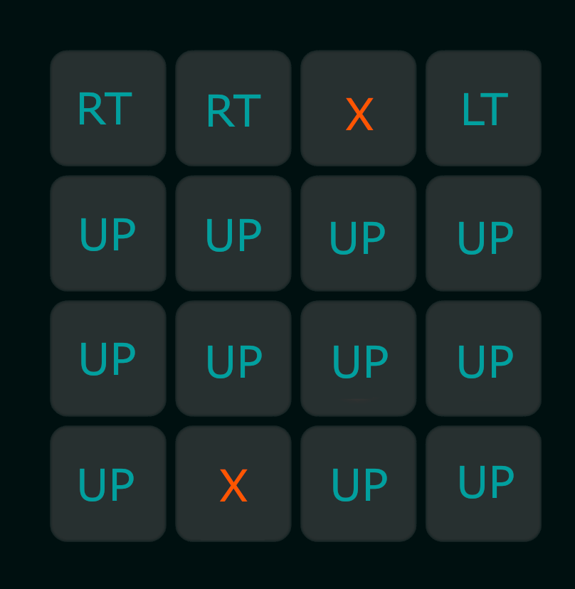
To build more intuition into what these observations and observations probabilities are, let us go back to the following example from class, where a robot tries to navigate a grid-world, but without information about where it is in the grid. Instead, the robot has a set of four sensors, that allow it to see whether there is an empty cell in each of the four cardinal directions. The colored cells denote obstacles in the image below.
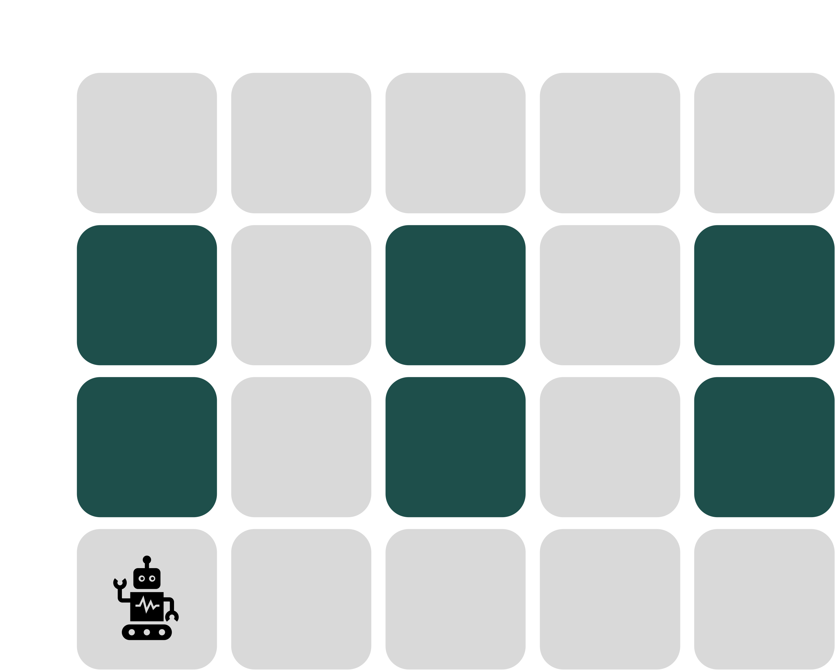
From any cell, an observation is simply what the robot's sensors return; an observation in this setting, therefore, is a binary vector of length 4, where each entry tells us whether there is an empty cell in that direction. Notationally, we will be following the order [UP, DN, LT, RT] to denote an observation. Consider the current shown position of the robot, i.e., the cell (3,0). The robot senses an obstacle/wall in the UP, DN and LT directions, but a free cell in the RT direction. The observation $O(s=(3,0))$ therefore is the binary vector [0,0,0,1].
Now consider a scenario where the robot's sensors may be faulty, and return an incorrect reading (i.e., a flipped bit) with some probability $p$. For now, let us assume the probability of a faulty reading from a given sensor is $0.1$. In this case, from a given cell, the agent may get more than one possible observation, as a result of one or more faulty sensor readings. Consider the same cell (3,0) as above. If all sensors work correctly, then the observation is [0,0,0,1]. However, if only the UP sensor fails, then the agent observes [1,0,0,1] instead. If instead, only the RT sensor fails, then we get [0,0,0,0]. If the UP and LT sensors fail, we get [1,0,1,1]. Similarly, through various combinations of sensor failures, the agent can observe all possible binary vectors of length 4 from each cell in the grid. However, not all of these observations are equally likely! For instance, to get the observation[1,1,1,0] from the cell (3,0), all four sensors on the robot would have to fail simultaneously! The probability of this happening is $0.1^4 = 0.0001$. In other words, the probability of getting the observation [1,1,1,0] from the cell (3,0) is $0.0001$. Similarly, the probability of observing [1,0,1,1] from cell (3,0) is $0.1\times0.9\times0.1\times0.9 = 0.0081$, since two sensors must fail and two others must function correctly to return this specific observation from this cell. These calcualtions are nothing but the observation probability $\Omega(s,o) = P(o|s)$.
Now, given an observation, the agent must update its belief about which state it is actually in, since the agent does not know this for sure. The belief state is defined as a probability distribution over the state space, representing the agent's likelihood of being in each state in the state-space. Since actions are still stochastic, instead of moving from state $s$ to $s'$, in a POMDP, the agent transitions between belief states, say $b$ to $b'$ as the result of an action $a$. This is known as the belief-state approach to solving POMDPs. To build intuition about this, let us consider the same grid-world POMDP as above. Let us assume the agent is in the (3,0) cell as before (although the agent does not know this), and makes the observation [0,0,0,1]. Now, we first need to compute the probability of the agent being in every cell in the grid-world, given this observation. Luckily, Bayes' theorem allows us to invert this dependency, and compute the probability as follows:
$$
P(s|o) = \frac{P(o|s)P(s)}{P(o)}
$$
where $P(o|s)$ is the probability of making the observation $o$ given the state $s$ - this is nothing but $\Omega(o,s)$, $P(s)$ is the prior probability of being in state $s$, and $P(o)$ is the probability of making the observation $o$. In the grid-world example, the prior probability of being in any cell at the beginning of time is $1/14$, since the agent has no information about its initial position and could be in any state. The denominator $P(o)$ is the probability of making the observation $o$ from any state, and is given by:
$$
P(o) = \sum_{s\in S} P(o|s)P(s)
$$
In practice, we can usually ignore the denominator, since it is the same for all states in the equation for $P(s|o)$, and only serves to normalize the belief state. Therefore, we can compute the belief state as:
$$
b(s) \propto \Omega(o,s)P(s)
$$
where $b(s)$ is the probability of being in state $s$ given the observation $o$. In the grid-world example, the belief state after making the observation [0,0,0,1] from the cell (3,0) is given by:
$$
b(s) \propto \Omega([0,0,0,1],s)P(s)
$$
This is computed for each cell $s$ in the grid world, and after normalization, results in the following probability distribution:
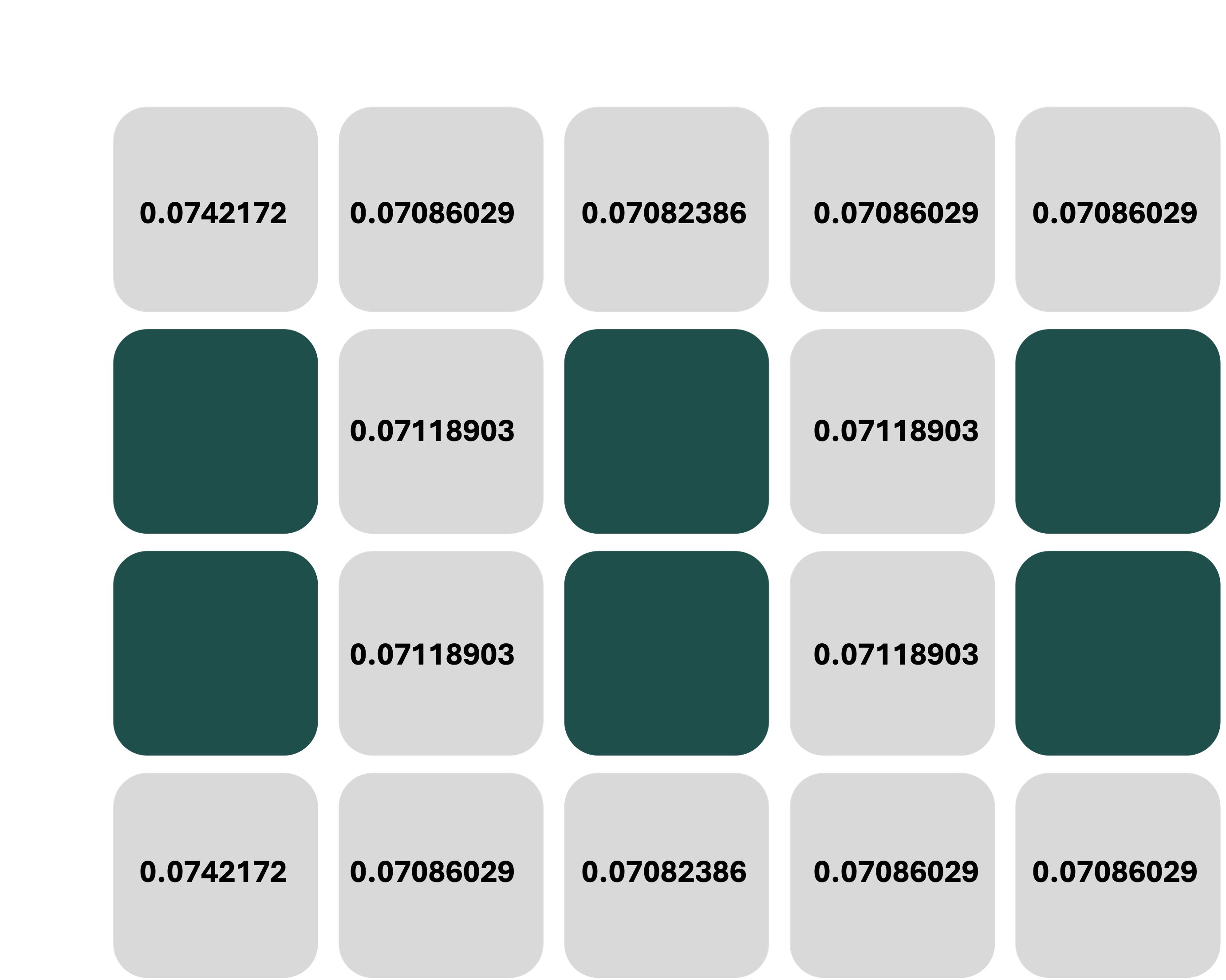
Now, assume the agent takes an action, say, a step towards the right, and receives a new observation, [1,0,0,1]. We can now begin to reason about the transition between belief states for POMDPs, instead of the transition model between states in standard MDPs. First, let us compute the belief state update resulting from this specific action and observation, and we will then discuss the belief state transition in general. The belief state update is given by: $$ b^{(t)}(s') \propto \sum_{s\in S} T(s,a,s')\Omega(o,s')b^{(t-1)}(s) $$ where $b^{(t)}(s')$ is the probability of being in state $s'$ after taking action $a$ and making observation $o$, and $b^{(t-1)}(s)$ is the last-known probability of being in state $s$ before taking action $a$. In the grid-world example, the belief state update after taking the action "right" and making the observation [1,0,0,1] from the cell (3,0) is given by: $$ b^{(t)}(s') \propto \sum_{s\in S} T(s,\textrm{right},s')\Omega([1,0,0,1],s')b^{(t-1)}(s) $$ There are a few key things to keep in mind here. First, note that we update the probability of being in every target cell $s'$, summing over all origin cells $s$ from where the action $a$ could have brought us to $s'$. This is opposite to the MDP Bellman equation, where we update the value of every origin state $s$, summing over all target states $s'$ under the action $a$. Second, just like the Bellman updates, the above belief-state update is calculated for every state in the state-space, considering each as a target state under the action $a$. Third, actions are stochastic, therefore we still have a notion of an action taking the agent to a different state than intended. In this example, let us assume that an action fails with probability $0.1$. If the action fails at a state where the only possible action is the valid action (such as the bottom left cell in the grid, and the 'right' action), then the agent stays in the same cell with probability $0.1$ and moves in the correct direction with probability $0.9$. If the action fails at a state where the agent can move in a different direction than intended (such as from the cell (3,1) under the 'right' action), then it moves in the correct direction with probability $0.9$, and one of the other directions (in this case, up or left) with probability $0.05$ each.
The complete calculation for the belief state update for all cells is best automated with code, but we show the update for one particular cell, say (3,1) as an example below:
$$
b^{(t)}((3,1)) \propto \sum_{s\in S} T(s,\textrm{right},(3,1))\Omega([1,0,0,1],(3,1))b^{(t-1)}(s)
$$
Now, we can plug in some known values into this equation. First, note that the possible states from which the agent could have reached $(3,1)$ under the 'right' action are its three neighbors, since actions are stochastic. Therefore, the sum over $s$ is essentially a sum over the set of states $\{(3,0), (3,2), (2,1)\}$. Next, we note that $\Omega([1,0,0,1],(3,1))$ is independent of $s$, and can be computed as we did earlier. The observation at $(3,1)$ if all sensors work correctly should be $[1,0,1,1]$; thus, in order to observe $[1,0,0,1]$, sensor 3 must have failed, and all others worked correctly. The probability of this occurrence is $0.1\times 0.9^3 = 0.0729$. Next, the transition probabilities $T(s,a,s')$ are the same as in the MDP, and can be computed from the rules of the grid-world. For instance, $T((3,0),\textrm{right},(3,1)) = 0.9$, $T((3,2), \textrm{right}, (3,1)) = 0.1$, since the agent can only slip into $(3,1)$ if the action fails from $(3,2)$ by design, and $T((2,1), \textrm{right}, (3,1)) = 0.1*0.5 = 0.05$, since the agent can slip either up or down from the cell $(2,1)$. Finally, the last-known belief state $b^{(t-1)}(s)$ is simply the set of values in the figure above, and we can substitute these into our update equation:
$$
b^{(t)}((3,1)) \propto 0.0729 * \bigg[ (0.9*0.0742172) + (0.1*0.07082386) + (0.05*0.07118903) \bigg] \approx 0.005645
$$
Similarly, we can update the belief state probabilities for every cell in our grid-world, and then normalize the belief state to get the final belief state after the action and observation. The original belief state, and the updated belief state after the action "right" and observation [1,0,0,1] are shown below:
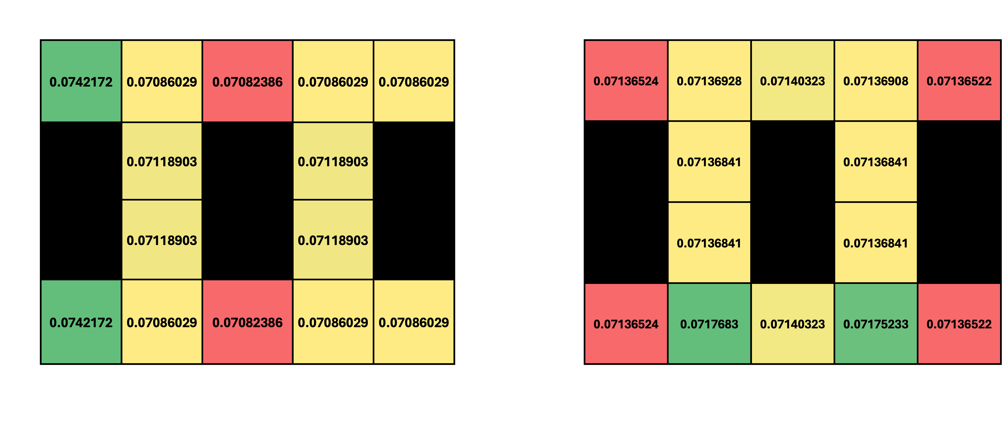
Green cells in each distribution denote the states with the highest probabilities, and red cells denote the states with the lowest probabilities. Note how the distribution of the agent's belief about its position has changed after the action and observation; specifically, the probability mass has shifted to the right, since the agent has made an observation that is somewhat consistent with the action it took.
The final step in our reasoning now has to do with the transitions between belief states, conditioned on an action. This is the POMDP equivalent of the transition model $T(s,a,s')$ in MDPs. In the case of POMDPs, we are looking for a transition model between belief states, i.e., $T(b, a, b') = P(b' | b, a)$. Note that this quantity is slightly different from the belief state updates we have done so far - we are now trying to estimate the probability of transitioning to one specific belief state (or probability distribution) from a previous one, given an action, accounting for all possible observations as a result of that action. We must keep in mind that unlike the number of states in an MDP, the number of belief states in a POMDP is infinite, since every probability distribution over the state-space is a valid belief state. However, given any one belief state, if we take an action and make an observation, we can only end up in one new belief state (just like what we did earlier, the two belief states in the above figure can be thought of as $b$ and $b'$ respectively).
To build intuition into this, let us consider the same grid-world example, and start by computing the probability of transitioning to a specific belief state from a previous belief state, given an action and observation. For instance, let us consider the transition from the belief state shown in the first figure above to the belief state shown in the second figure, given the action "right" and observation [1,0,0,1]. This transition is given by: $$ T(b, \textrm{right}, b') = P(b' | b, \textrm{right}) $$ Since the agent transitioned into some state $s'$ as the result of the action $a$ (despite our uncertainty), we can compute this transition by accouting for all possible transitions $s$ to $s'$. Since we are now not given an observation, we must also account for all possible observations $o$, and therefore sum over $o$ as well: $$ T(b, \textrm{right}, b') = \sum_o \sum_{s'} P(b', o ,s' | b, \textrm{right}) $$ This is the probability of transitioning to the belief state $b'$, given the action "right" and the previous belief state $b$. By summing over all $o$, we account for every possible observation the agent may receive (doing this takes care of faulty sensors for instance), and summing over $s'$ accounts for every state the agent might end up in, starting from some state $s$ as defined by our previous belief state. We can expand this as follows using the chain rule of conditional probability: $$ T(b, \textrm{right}, b') = \sum_o \sum_{s'} P(b' | o, s', b, \textrm{right})P(o | s', b, \textrm{right})P(s' | b, \textrm{right}) $$ Now note that $P(b'|o,s,b,\textrm{right})$ is the probability of a specific belief state, given the previous belief state, an action, an observation, and the new state $s'$. However, since $b'$ itself is a distribution over all $s'$, we can drop that dependency from the conditional. Similarly $P(o|s',b,\textrm{right})$ is the probability of making the observation $o$ given the state $s'$ and the action $a$. However, observations only depend on $s'$, hence we can drop the dependency on $b$ and $a$, and this term turns out to be nothing but $\Omega(o,s')$. This reduces our equation to: $$ T(b, \textrm{right}, b') = \sum_o P(b' | o, b, \textrm{right})\sum_{s'}\Omega(o,s') P(s'|b,a) $$ Finally, $P(s'|b,a)$ is the probability of transitioning to state $s'$ from the previous belief state $b$ under the action $a$. To calculate this, we simply need to multiply each transition probability $T(s,a,s')$ by the probability that the agent was indeed in state $s$, which is nothing but $b(s)$; and sum over all states $s$, since we are uncertain about the agent's actual position. Our transition equation finally becomes: $$ T(b, \textrm{right}, b') = \sum_o P(b' | o, b, \textrm{right})\sum_{s'}\Omega(o,s') \sum_s T(s,a,s') b(s') $$ We can now plug in known values for the transition probabilities, observation probabilities, and the previously computed belief state. However we still need to deal with the first term, $P(b'|o,b,\textrm{right})$. Now recall that this is the probability that the agent was in belief state $b$, took the 'right' action, observed $o$ and ended up in $b'$. From our previous belief state update (shown in the figure with two distributions above), we know that from a particular $b$ (say the distribution on the left), for a particular action and observation, we transition to exactly one new belief state $b'$ (the distribution on the right). Therefore, $P(b'|o,b,\textrm{right}) = 1$ if the action and observation indeed lead to the new belief state under consideration, and $0$ otherwise.
We now have the following quantities, using which a POMDP can be represented as an MDP over belief states:
- Space of Belief States, $B$ : probability distributions over the state space, representing the agent's likelihood of being in each state in the state-space.
- Action Space, $A$ : Same as MDPs.
- Reward Function, $R(b, a, b')$ : the expected reward of transitioning from a previous belief state to a new belief state, given an action.
- Belief State Transition Model, $T(b, a, b')$ : the probability of transitioning to a specific belief state from a previous belief state, given an action and observation.
- Discount Factor, $\gamma$ : same as MDPs.
For further reading on tractable methods to solve POMDPs, please refer to POMDP.org - a POMDP tutorial.
Reinforcement Learning
As our final layer of complexity, imagine a situation where neither the transition probabilities nor the rewards are known a priori. The action space is assumed to be fully known, and the state space may or may not be fully known. In such environments, we deploy a class of algorithms known collectively as reinforcement learning (RL), where the agent learns to make decisions through interactions with the environment. The agent may choose to infer or estimate the underlying mechanics of the world such as $T(s,a,s')$ and $R(s,a,s')$, or directly try to optimize the value function in search of an optimal policy. We will now discuss both these approaches.
Consider the following simulation of our 100-sided die-rolling game from class, where you, the agent, chose from action A or B, and the game environment (the prof.) would return a reward, and inform you whether the game is ended. The only information that you, the agent, must rely on is the reward and the fact that the game is still ongoing. The agent must then learn to make decisions based on this limited information.
From the gameplay, we can first infer that there are 2 states in the game, the start state S and the absorbing state END. TERMINATED state is not really a state; rather, it refers to the case where after some set number of moves, the environment is programmed to end a round of the game prematurely, and start the next round or episode. Given the two action choices A and B, we can see that both actions may bring an agent that starts in S back to S, but only A can take the agent to the END state. We can also observe that any transition back to the start state has a reward of $-1$, and the transition to the end state has a reward of $+100$. For now, we assume that the reward for a given transition does not change between or in the middle of episodes. This information yields the following MDP:
Now, all that remains is to infer the transition probabilities. Looking back at the data, since we never observed the action B leading our agent to the end state, we may estimate that $T(S, B, END) = 0$. Of course, this estimate may be incorrect, since it is based on a limited amount of information from a very small number of episodes. However, as the number of episodes increases, this estimate will become more and more accurate. Similarly, we can see that when aciton A is played, out of 115 times, the agent ended up back in the start state 111 times, and 4 times in the END state. We may, therefore, estimate that $T(S, A, S) = \frac{111}{115} = 0.965$ and $T(S, A, END) = \frac{4}{115} = 0.035$.
Such an approach is called Model Based Monte Carlo (MBMC) estimation, since we assume an underlying MDP, and use the data solely to infer the model's parameters, namely the transition probabilities and rewards. Once we have an MDP, evaluating a given policy, or computing the optimal policy proceeds exactly as we did before. However, this approach may have a few drawbacks. Before you read the next section, pause and think about what these drawbacks may be.
- The first drawback is that MBMC approaches use data-based estimates to construct a fixed model of the environment. Once this model is constructed, it is typically not updated, but is instead assumed to be a 'good enough' representation of the environment. Of course, implementing running updates of the transition probabilities is no big feat of mathematics; but that, in turn, leads us nicely to the second drawback.
- The second drawback is that policy evaluation and optimal policy estimation for a given MDP is mathematically (or computationally, for us CS majors) expensive, since we rely on iterative algorithms based on the Bellman update equation. Recall that to compute optimal policies, we must consider all possible actions from all states, running a large number of updates for each legal state-action pair until the values converge. After having gone through all that trouble, imagine we now have to update our MDP based on new data. Immediately, the previously computed optimal policies must be discarded and re-computed from scratch, since our estimated transition probabilities have now changed.
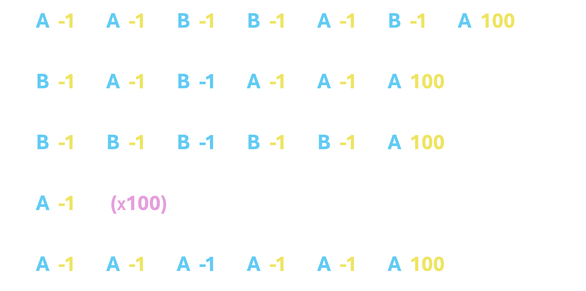
Let us start with the easiest possible variant; where we already have data gathered from a number of episodes. Consider the same data we used earlier, gathered by playing the dice game simulation above for 5 episodes.
However, this time, instead of counting the number of times a given transition occurs and recording the reward, we shall dig a little bit deeper into the information each episode is giving us. First, recall what a Q-value for a state-action pair represents: it is the expected value of taking a specific action $a$ from a state $s$, and then continuing to play the game by following some underlying policy $\pi$. (If this concept is unclear to you, it would be worth revisiting the section on MDPs. Please reach out to the TAs or the instructor if you need further clarification.)
Now, let us look at the first episode alone, and reason about what this data tells us about $Q_\pi($S, A$)$ - the expected value of being in the start state, and choosing action A.

Recall that this expected value, $Q_\pi($S, A$)$ consists of two sets of rewards: immediate rewards as a result of a transition into a next state $s'$ by taking the action A, and a discounted future reward, accounting for everything else that happens thereafter. In the above episode, action A is the very first action our agent takes, ends up back in S, and gets an immediate reward of $-1$. The rest of the episode contributes to the discounted future reward portion of the expected value.
Assuming the discount factor, $\gamma=1$ for simplicity, the 'future reward' of taking action A from state S is $95$. Thus, the utility of taking action A from state S is $-1 + 95 = 94$. Let us call this $u_1($S, A$)$. We now repeat this process for all episodes; starting from the first time we encounter the pair S, A, we compute the utility, $u_t($S, A$)$ for each episode that the pair occurs, we consider the immediate and discounted future rewards. Finally, we say that $Q_\pi($S, A$)$ is the average of the computed utilities. The following image illustrates this computation:
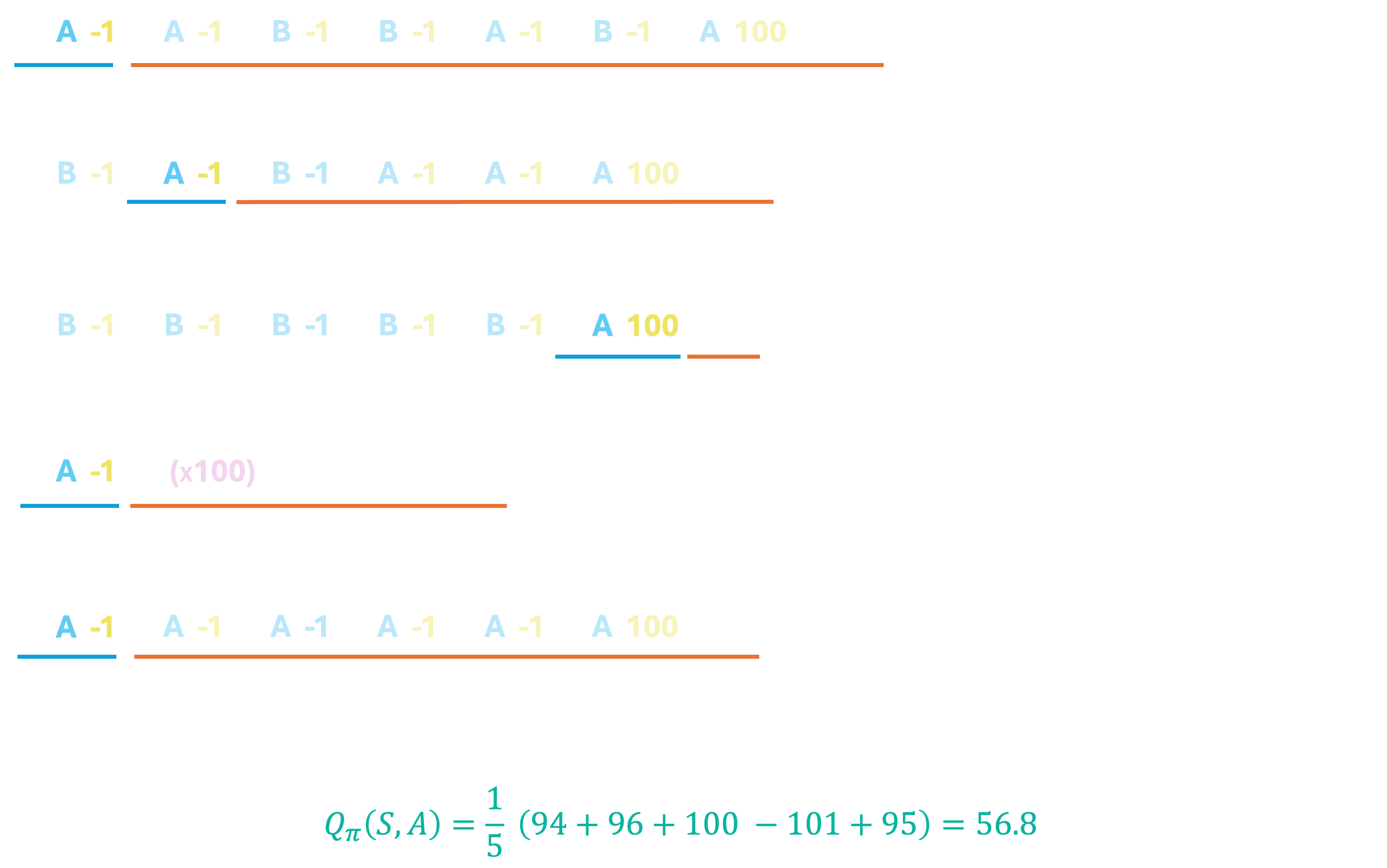
We only consider the first occurrence of the state-action pair that we are interested in, in each episode - and the utility is computed as a discounted sum over the remainder of the episode. This is simply to avoid double counting rewards - note that the immediate reward of $-1$ when taking action A for the second time in the first episode already features in the future rewards for the same action taken earlier, albeit with a discount factor. Following a very similar, process, we can also compute $Q_\pi ($S, B$)$, which turns out to be $95.\overline{33}$. It would be a good idea to write out the steps for this on your own and compare our final solutions to check your understanding. (HINT: for $Q_\pi($S, B$)$, completely ignore all episodes where the pair does not occur at least once.)
Compare what we just did to a model-based approach. Upon receiving data from a new episode, in a model-based approach, we would first need to update transition probabilities, then run several iterations of Bellman updates to approximate Q-values for each state-action pair. Instead, in a model-free approach, we directly approximate Q-values by averaging over episode-wide utilities. Upon receiving data from a new episode in a model-free approach, we simply need to update our average utility for each state-action pair that occurred in this new episode.
Although this is an improvement over MBMC, we can do better still. There are two questions that naturally arise with this approach, that we would benefit from addressing:
- What do we do about the incredibly high variance in the utilities between episodes?
- How do we maintain a running average of utilities (which is the Q-value) without explicitly storing all past values?
The answer to the first question is somewhat straightforward, especially to those who may have experience with dynamic programming. In Reinforcement Learning, Bootstrapping refers to the process of updating estimates of the value function based on the estimated value of subsequent states or actions, rather than waiting for the final outcome (like the end of an episode). Perhaps a more intuitive phrasing of that process could be: When an agent takes an action $a$ from a state $s$, and ends up in a new state $s'$, we use our best guess about what happens thereafter (based on what we already know about $s'$) instead of actually playing out the rest of the episode to make an update to $Q_\pi(s,a)$. This, in turn, leads us to a new class of RL algorithms, collectively known as Temporal Difference methods.
Let's break that down; let's assume our agent starts in state $s$, takes action $a$, receives reward $r$, and ends up in state $s'$. To compute the utility for this state-action pair, we first account for the immediate reward, which is simply $r$ as returned by the environment. Now, instead of computing discounted future rewards as a weighted sum over the actual rewards obtained from the rest of the episode, we shall instead rely on our best estimate of what happens next. Where do we get this estimate from? Recall that the Q-value of a state-action pair is simply the expected utility of being in that particular state and taking that particular action, and then continuing to follow a policy $\pi$. Therefore, given a next action $a'$ that the agent takes from $s'$ (which is where it currently is), we can use the value $Q(s',a')$ as an approximation for what happens in the rest of the episode. While at the beginning of training, we do not have a reasonable estimate of $Q_\pi$ for any state-action pair, we can overcome this problem with an iterative algorithm that works very similarly to our iterative Bellman updates in MDPs, where we start by simply assuming that $Q_\pi$ for all state-action pairs is initially $0$.
This approximation serves a dual purpose: a) it helps reduce variance between updates to $Q_\pi(s,a)$, since much of the variance arises as a result of differences in episode length (time-to-termination), owing to the randomness associated with the underlying policy $\pi$; and b) it allows us to make an update to $Q_\pi(s,a)$ for every observed set of $(s, a, r, s', a')$, instead of one update per episode, reducing overall wait time between updates. These factors combined, in practice, also lead to a faster convergence to a stable (and accurate) estimate of the value function. In other words, we can get away with fewer episodes of gameplay to generate an overall accurate estimate of the Q-function, compared to when we were doing one update per episode.
Before we work through an example, we must first solve the second problem - that of maintaining running averages without storing entire value histories. We turn to convex combinations (linear combinations where coefficients sum to 1), where the coefficients are determined by the number of updates to a given value. Forget about Q-values for a bit, and just think of the following sequence of numbers: $1, 2, 3, 4, 5$. The mean of these numbers is, of course, $3$. Now imagine if instead of all five numbers in the sequence being presented at once, we were given the numbers one at a time, and asked to update our estimated mean. At time $t=1$, we would see the first entry in the sequence, the number $1$, and that would be our estimated mean. At time $t=2$, we would observe the value $2$, and would update our mean as $\frac{1+2}{2} = 1.5$. At time step $t=3$, we would update our estimated mean as $\frac{1+2+3}{3} = 2$. Now pause, and try to answer the following question: instead of using the actual values $1, 2$ and $3$ to compute the updated mean at $t=3$, can we somehow combine our previous estimated mean ($1.5$) from $t=2$ and the new data point ($3$) to come up with the updated mean of $2$?
Remember that two values ($1$ and $2$ respectively) contributed to the previous estimate of the mean ($1.5$), and we have one new data point (the value $3$) to account for. To update our mean then, we simply need to take a weighted average of the previous estimate of the mean and the new data point, where the weights depend on the number of terms that contributed to each of the terms. For this example, $\frac{2}{3}\times 1.5 + \frac{1}{3} \times 3 = 2$. Now extend this reasoning to the next timestep. Our mean after observing three terms is $2$, and the next data point we observe is $4$. Our weights would therefore be $\frac{3}{4}$ for our estimated mean (since it was estimated after observing three terms out of four), and $\frac{1}{4}$ for the new data point. Thus, our updated mean can be computed as $\frac{3}{4}\times 2 + \frac{1}{4}\times 4 = 2.5$. In fact, this reasoning can also be applied for the very first estimate of the mean as well - imagine that your estimate at $t=0$ is simply $0$, since nothing has been observed so far. After observing the value $1$ at $t=1$, the weights are $0$ for the current estimate, since no observed terms contributed to our guess of $0$, and $1$ for the new observed data point; and $0\times 0 + 1\times 1 = 1$.
Note that in all of these updates, the coefficient for the previous estimate and that of the new observed value always add up to 1 (hence a convex combination). The updates, therefore, may be written as a general equation based on the number of updates. Let $\hat{\mu}$ be our estimated mean. Let the initial estimate based on no data be $\hat{\mu} = 0$. Then, for each observed data point $d$, we may update $\hat{\mu}$ as follows: $$ \begin{align*} \eta = &\frac{1}{1 + \textrm{number of completed updates to}\ \hat{\mu}}\\\\ &\quad\quad\quad\quad\hat{\mu_t} = (1-\eta) \hat{\mu}_{t-1} + \eta d\\ \end{align*} $$ where the $t-1$ and $t$ subscripts simply indicate the previous and updated values of the estimate respectively.
Finally, to recycle a metaphor from the 17th century, combining these two ideas (bootstrapping and convex combinations) finally gives us the SARSA algorithm, the stone that kills two birds. To maintain a running estimate of $Q_\pi(s,a)$ without waiting for episodes to end, or storing the entire history of the estimated value, we make an update to $Q_\pi(s,a)$ every time we observe the action $a$ being taken from state $s$, by looking one step ahead and considering the next state $s'$ and the subsequent action $a'$. Here's a summary of how the algorithm works:
The SARSA Algorithm
For each observed $(s, a, r, s', a')$,
\[\eta = \frac{1}{1 + \textrm{number of completed updates to}\ Q_\pi(s,a)}\]
$Q^{t}_\pi = (1-\eta)Q^{t-1}_\pi + \eta (r + \gamma Q_\pi(s', a'))$
Increase number of completed updates to $Q_\pi(s,a)$ by 1.
Let us run through an example. Consider the same set of five episodes we previously used, except this time, we will use SARSA to estimate the Q-values, $Q_\pi($S, A$)$ and $Q_\pi($S, B$)$. Note that these are the only two legal (observed) combinations, since the only other state the agent can be in is the END state, from where no further actions are possible. One final nuance here, is that we need to track the number of updates to the Q-value for each state-action pair separately. We therefore initialize our Q-table, and update counter table as follows:
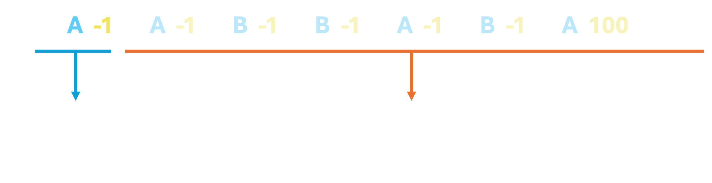
Now, every time we observe a sequence of $(s, a, r, s', a')$, we use the equation from the SARSA algorithm to update the Q-table. Let's start with the first episode. The first observed sequence of $(s, a, r, s', a')$ is highlighted below:

Since the agent takes action A from state S, we get to update the entry corresponding to $Q_\pi($S, A$)$. To do so, we first calculate $\eta$ using the number of times $Q_\pi($S, A$)$ has been updated so far, which is $0$. Thus, \[\eta = \frac{1}{1+0} = 1\]
Next, we note that the agent ended up in $s'=$S, and took the subsequent action $a'$=A. Thus, we look up the corresponding $Q_\pi(s', a')$ value to use as a proxy for our discounted future reward, which is also currently $0$. Finally, we run the update equation, assuming $\gamma=1$ for simplicity:
$$
\begin{align*}
Q_\pi(\textrm{S, A}) = (1-\eta) \times 0 + \eta\times [r + \gamma\ Q_\pi(\textrm{S, A})]\\
= (1-1) \times 0 + (1) [-1 + (1\times 0)]\\
= 0 + (-1)\\
= -1
\end{align*}
$$
Therefore, our updated Q-table and update-counter table are as follows:
Let us walk through two more updates, to make sure our understanding is correct: the next observed $(s,a,r,s',a')$ sequence is highlighted below:

The value of $\eta$ is now calculated as $\frac{1}{1 + 1} = \frac{1}{2}$. This gives us the following update:
$$
\begin{align*}
Q_\pi(\textrm{S, A}) = (1-\eta) \times -1 + \eta\times [r + \gamma\ Q_\pi(\textrm{S, B})]\\
= (1-\frac{1}{2}) \times -1 + \frac{1}{2}[-1 + (1\times 0)]\\
= -0.5 + -0.5
= -1
\end{align*}
$$
Now, our updated Q-table and update-counter table are as follows:

The next observed $(s,a,r,s',a')$ sequence is highlighted below:

The value of $\eta$ is now calculated as $\frac{1}{1 + 0} = 1$, since $Q_\pi($S, B$)$ has never been updated before. This gives us the following update:
$$
\begin{align*}
Q_\pi(\textrm{S, B}) = (1-\eta) \times 0 + \eta\times [r + \gamma\ Q_\pi(\textrm{S, B})]\\
= (1-1) \times 0 + (1) [-1 + (1\times 0)]\\
= 0 + (-1)\\
= -1
\end{align*}
$$
Now, our updated Q-table and update-counter table are as follows:
This process is then continued, moving on to the next observed $(s,a,r,s',a')$ sequence, making one corresponding update, and so on. Note that we only update the Q-value (and update counter) for the specific $s,a$ pair featured in each observed $(s,a,r,s',a')$ sequence. Continue this process on your own, and see what final estimate you get after processing the remaining episodes in this example. Also note how the estimated values of $Q_\pi$ for any given state-action pair don't fluctuate as wildly between updates as they did before (when we made updates after each episode).
So far, we have assumed that the data is generated by some underlying policy $\pi$, and that is the same policy for which SARSA computes the expected values. SARSA, therefore, is an example of an on-policy learning technique. However, the key motive in training an agent in a reinforcement learning setting is for the agent to eventually figure out an optimal policy - the state-action mapping that maximizes the expected utility. To this end, we now dive into off-policy learning, where the agent learns the expected value for the optimal policy while using a completely different policy to explore the environment. The policy used to explore the environment is often referred to as an exploration policy.
So how do we learn $Q_{opt}(s,a)$ for some state-action pair while using a different exploration policy $\pi(exp)$ to explore the environment? If you think back to MDPs, the answer to this question is, in fact, a very similar modification to the SARSA algorithm. In the update equation for $Q_{opt}(s,a)$, instead of using $Q_{\pi(exp)}(s', a')$ as a proxy for the discounted future reward, we use $V_{opt}(s') = \max_{a'} Q_{\pi(exp)}(s', a')$ as a proxy instead. This gives us the following algorithm to infer optimal expected utilities:
The Q-Learning Algorithm
For each observed $(s, a, r, s')$,
\[\eta = \frac{1}{1 + \textrm{number of completed updates to}\ Q_{opt}(s,a)}\]
$Q^{t}_{opt} = (1-\eta)Q^{t-1}_{opt} + \eta (r + \gamma V_{opt}(s'))$
Increase number of completed updates to $Q_{opt}(s,a)$ by 1.
Let us go back once again, to the same five episodes, and walk through a few updates, this time estimating the optimal expected values. One key thing to note here, is that the data was not generated by playing optimally: in fact, it was generated by a completely different exploration policy that changed with each episode. This is the beauty of off-policy learning - the ability to extract the optimal expected value function from this data, in turn giving us the optimal policy. We will see later that separating the exploration policy in this manner has some added benefits.
As opposed to SARSA, in the Q-learning algorithm, we are interested in sequences of $(s,a,r,s')$, and we don't look ahead at the subsequent action $a'$ taken by the agent. Instead, we will consider all possible actions that the agent could have taken from $s'$, and pick the maximizing expected value. First, we initialize our Q-table and update counter, just as we did for SARSA, but this time, the entries in the Q-table correspond to $Q_{opt}$, and not $Q_\pi$ (or to be more precise, $Q_{\pi(exp)}$ in this setting).
Now, every time we observe a sequence of $(s, a, r, s')$, we use the Q-learning equation to perform an update to our Q-table. Let's start with the first episode. The first observed sequence of $(s, a, r, s')$ is highlighted below:

Just like SARSA, since the agent takes action A from state S, we update the entry corresponding to $Q_{opt}($S, A$)$. To do so, we first calculate $\eta$ using the number of times $Q_{opt}($S, A$)$ has been updated so far, which is $0$. Thus, \[\eta = \frac{1}{1+0} = 1\]
Next, we note that the agent ended up in $s'=$S, but this time we don't look at the subsequent action $a'$=A in particular. Instead, we look up the maximum value from the row corresponding to state S in the Q-table to use as a proxy for our discounted future reward, which is also currently $0$. Doing so accounts for all possible actions that could have been taken from the state S, and the largest value from this row is nothing but $V_{opt}($S$)$. Finally, we run the update equation, assuming $\gamma=1$ for simplicity:
$$
\begin{align*}
Q_{opt}(\textrm{S, A}) = (1-\eta) \times 0 + \eta\times [r + \gamma\ V_{opt}(\textrm{S})]\\
= (1-1) \times 0 + (1) [-1 + (1\times \max\{0, 0\})]\\
= 0 + (-1)\\
= -1
\end{align*}
$$
Therefore, our updated Q-table and update-counter table are as follows:

The next observed $(s,a,r,s')$ sequence is highlighted below:

The value of $\eta$ is now calculated as $\frac{1}{1 + 1} = \frac{1}{2}$. This gives us the following update:
$$
\begin{align*}
Q_{opt}(\textrm{S, A}) = (1-\eta) \times -1 + \eta\times [r + \gamma\ V_{opt}(\textrm{S})]\\
= (1-\frac{1}{2}) \times -1 + \frac{1}{2}[-1 + (1\times \max\{-1, 0\})]\\
= -0.5 + -0.5
= -1
\end{align*}
$$
Now, our updated Q-table and update-counter table are as follows:
The next observed $(s,a,r,s')$ sequence is highlighted below:

The value of $\eta$ is now calculated as $\frac{1}{1 + 0} = 1$, since $Q_{opt}($S, B$)$ has never been updated before. This gives us the following update:
$$
\begin{align*}
Q_{opt}(\textrm{S, B}) = (1-\eta) \times 0 + \eta\times [r + \gamma\ V_{opt}(\textrm{S})]\\
= (1-1) \times 0 + (1) [-1 + (1\times \max\{-1, 0\})]\\
= 0 + (-1)\\
= -1
\end{align*}
$$
Now, our updated Q-table and update-counter table are as follows:
Even though we arrived at the same values in our $Q_{opt}$ computation as we did for $Q_\pi$ earlier, it is important to recognize that we did so through a slightly different process, and this is simply a coincidence. As you continue to update Q-values using either method, you may see differences emerge in the respective Q-tables, owing to the fact that Q-learning always uses the maximum expected utility from the resulting state $s'$, whereas SARSA uses the expected utility tied to the next action observed in gameplay.
Finally, let's think about how to decide the exploration policy $\pi(exp)$. First, keep in mind that we use the data generated by the exploration policy to in turn, infer the optimal policy (referred to as exploitation in RL literature) - which implies that we should incentivize choosing good moves in general, to at least some degree. However, at the beginning of gameplay, the agent does not have an accurate view of the world; in other words, we don't really know which moves are optimal. On the other hand, there is also value in taking random actions, which allows us to explore the state-space more thoroughly as we try all the various combinations of state-actions pairs possible. With more random actions, there is a higher likelihood that the agent will observe rewards for most, if not all transitions in the underlying MDP.
One popular technique ussed to account for these opposing objectives (exploration v/s exploitation) is the $\epsilon$-greedy approach. The policy in this setting is no longer a static mapping of one action to each state; instead, the policy is a probability distribution over all valid actions that the agent may take from each state. Further, this distribution itself is not static, but changes over time - starting off by encouraging exploration more, in order to gather information about as many state-action pairs and transitions as possible, but gradually shifting to favor exploitation, i.e., making more optimal moves. Formally, a policy for a state $s$ using the $\epsilon$-greedy approach is defined as follows:
Let $\epsilon$ be the probability of taking a random action, and be initialized to a number close to or equal to $1$. At each timestep: \[ \pi(s) = \begin{cases} \textrm{random action with probability } \epsilon, \\ \textrm{optimal action, } \arg\max_a Q_{opt}(s, a) \textrm{ with probability }(1-\epsilon) \end{cases}\] After taking an action based on the above probabilities, we reduce $\epsilon$, typically by multiplying it by a constant decay factor less than $1$, which is nothing but an exponential decay in the probability of taking a random action over time. As $\epsilon$ decays to a value close to $0$, $\pi(exp)$ converges to $\pi_{opt}$, and if the exploration was thorough enough, we should have at the end, an agent that has learnt to maximize reward in its environment by taking optimal actions from each state.